Monitoring Signals for Degradation, Alerting, Diagnosis, and Retraining

Hello. In the previous lesson, you designed a release process that uses shadowing, canaries, promotion gates, and rollback. Those mechanisms protect the system during a change. Monitoring is the longer-running control loop: it tells the team whether the serving system remains available, whether its inputs still mean what the model expects, and whether its decisions remain useful after deployment.

This lesson gives you an interview-ready way to define service, data, and model signals, then connect a detected degradation to the right alert, investigation, and remediation. The central discipline is simple: a metric is valuable only when it supports a decision.

---

Monitoring is a decision system, not a dashboard collection

Monitoring collects and displays operational evidence. But a production ML system needs more than charts: it needs an agreed response when evidence changes.

For each signal, define five things:

1. What is measured?
   For example, p95 inference latency, feature missingness, recall, or the fraction of predictions above a decision threshold.

2. What baseline is used?
   This could be the training distribution, a known-good production period, the incumbent model, or a seasonally comparable period.

3. What constitutes concerning change?
   Use a threshold, a rate of change, or a statistical test, with a minimum sample size and time window.

4. Who owns the response?
   Platform/SRE may own serving availability; a data-producing team may own an upstream feature; the model team may own performance investigation.

5. What action follows?
   Actions differ: rollback, route to a fallback, repair a pipeline, pause promotion, collect labels, retrain, or simply continue observing.

This distinguishes a monitoring signal from an alert. A signal is a measurement. An alert is a request for someone to act. Every page should correspond to an urgent, actionable situation; otherwise, engineers become desensitized to alarms.

The monitoring loop has three connected layers:

Layer	Core question	Example evidence	Typical immediate action
Service monitoring	Can the system serve valid predictions reliably?	Error rate, latency, throughput, saturation	Scale, fail over, rollback, repair dependency
Data monitoring	Are inputs valid, fresh, and comparable to expectations?	Schema violations, missingness, feature drift, training-serving skew	Quarantine data, activate fallback, investigate source
Model monitoring	Are predictions and real-world outcomes still acceptable?	Calibration, precision/recall, business outcome, slice performance	Investigate, gather labels, retrain and validate a candidate

The layers are deliberately separate because a poor business outcome does not necessarily mean “the model needs retraining.” A feature pipeline might be emitting nulls. Conversely, perfectly healthy infrastructure does not prove that predictions remain useful.

---

Service signals: first establish that inference works

An ML endpoint is still a service. If it is unavailable, slow, overloaded, or returning malformed responses, model quality is irrelevant because users cannot obtain a usable decision.

Google’s SRE guidance calls out four core signals: latency, traffic, errors, and saturation.

For an online prediction service, a practical initial service dashboard might include:

Signal	How to segment it	Why it matters
Availability / valid-response rate	Model version, endpoint, region, client	Captures whether a prediction is actually delivered
Latency	p50, p95, p99; successful and failed requests separately	Protects the user experience and exposes dependency degradation
Traffic	Requests per second, concurrent requests, queue depth	Detects demand shifts and supports capacity planning
Errors	Status code, error class, model version, dependency	Separates invalid requests from model-loading or feature-store failures
Saturation	CPU, memory, GPU utilization, queue lag, connection pools	Warns that performance may deteriorate before hard failure
Dependency health	Feature-store latency, cache hit rate, upstream timeout rate	A model endpoint often fails because a dependency failed

Use an ML-specific definition of a successful response

A successful HTTP response is not always a successful prediction. A service can return status 200 while producing a default score because a critical feature lookup failed. For high-impact systems, define a valid prediction with explicit conditions, such as:

• the request passed schema validation;
• required features were present or an approved fallback was used;
• the model artifact loaded successfully;
• the response was produced within the committed latency policy;
• the output passed basic validity checks, such as being finite and within an allowed range.

This is an example of combining black-box and white-box monitoring. External synthetic requests can test whether the endpoint returns an expected response. Internal telemetry can reveal whether that response relied on stale features, a fallback path, or a degraded downstream dependency.

Make service alerts actionable

A useful severity policy might look like this:

Condition	Notification	Likely owner	First action
Sustained user-visible error or severe SLO breach	Page	Platform or serving on-call	Fail over, rollback, mitigate dependency
Rising p99 latency with high saturation but no user breach yet	Ticket or urgent chat alert	Platform team	Scale, inspect queue and dependency pressure
Candidate version has elevated errors during canary	Automated release gate plus page if severe	Release owner and platform on-call	Halt promotion; rollback candidate if threshold is breached
One isolated timeout or short traffic spike	Dashboard only	None initially	Observe and correlate with other signals

The alert condition should specify scope and duration. A single failed request is data for a dashboard; a sustained high error rate across production traffic might be a page. Similarly, a high p99 latency for five minutes during a low-traffic period may be statistically unstable; define a minimum request count before treating it as evidence.

---

Data signals: verify the world reaching the model

A deployed model makes assumptions about inputs: their types, ranges, distributions, meanings, and availability at prediction time. Data monitoring tests whether those assumptions still hold.

Google’s production ML guidance separates raw-data validation, feature validation, slice analysis, training-serving skew, and checks of live model quality.

Data quality is not the same as data drift

Start with data quality and contract signals. These detect inputs that are invalid, incomplete, late, or structurally incompatible:

• schema-validation failures;
• feature type changes;
• missing or null-value rate;
• range violations, such as a negative account age;
• new or unknown categorical values;
• duplicate, malformed, or impossible records;
• feature freshness and source-ingestion lag;
• volume anomalies, such as a sudden 90% reduction in requests from one region.

These are often operational defects, not model-decay events. If a frontend update suddenly sends null income values to a lending model, retraining on the corrupted data would make the situation worse. The immediate response is to stop or isolate the bad input, activate a safe fallback if one exists, and investigate the producer contract.

Next, monitor feature-engineering health. Raw input may pass validation while the transformed feature vector is incorrect. Check, for example:

• transformed numeric ranges and clipping rates;
• the fraction of features populated by defaults;
• one-hot encoding validity;
• changes in feature computation failures;
• online/offline feature consistency;
• feature-store retrieval latency and freshness.

A particularly important class is training-serving skew:

• Schema skew occurs when training and serving inputs no longer conform to the same expected schema or data assumptions.
• Feature skew occurs when the engineered values differ between training and serving, perhaps because transformations diverged or an online feature was computed with different timing.

Both can make an offline evaluation look excellent while production performance deteriorates.

Drift is an early-warning signal, not a verdict

Data drift means the distribution of incoming inputs differs from the chosen reference distribution. For a feature $X$, this is a change in $P(X)$. For example, a demand model may see a different mix of regions, products, or customer types than it saw in training.

You can compare reference and current distributions with measures such as Population Stability Index, Kolmogorov-Smirnov tests, KL divergence, or Jensen-Shannon distance. The metric itself is less important than choosing an interpretable method, a valid baseline, sensible windows, and thresholds calibrated to the feature’s business importance.

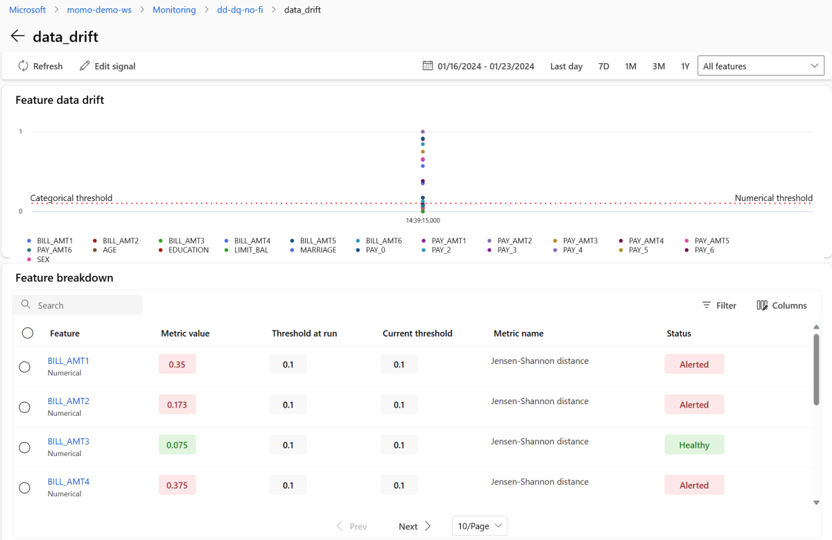
The dashboard in the image illustrates an important management principle: do not alert only on an aggregate “drift score.” A broad distribution shift might be expected after a planned marketing campaign; a large shift in a safety-critical feature may be urgent. Monitor:

• drift by individual feature;
• the count and proportion of drifted features;
• drift in critical features separately;
• drift by business-relevant slice;
• whether prediction scores or decision rates changed at the same time.

A detected distribution change does not prove that the model is worse. If a recommendation model begins serving more users in a new country, feature distributions should change. The question is whether the model’s behavior and eventual outcomes remain acceptable for that new population.

---

Model signals: test predictions against reality where possible

Model monitoring is about the quality and consequences of decisions, not merely whether a model process is running.

The strongest model-quality signals require labels. Once ground truth arrives, compare predictions to outcomes over a defined window. The appropriate metrics depend on the product objective:

Problem type	Model-quality signals	Business or risk companion signal
Binary classifier	Precision, recall, false-positive rate, false-negative rate, calibration	Fraud loss, manual-review load, harmful decisions
Ranking or recommender	Ranking quality, click or conversion outcomes, coverage	Engagement, retention, marketplace health
Regression	MAE, RMSE, bias, error percentiles	Forecast error cost, stockouts, overprovisioning
Human-in-the-loop system	Override rate, reviewer disagreement, abstention rate	Review workload, time to decision, escalation rate

Track these metrics by model version, data/feature version, serving configuration, and important slices. A global precision value can conceal a severe decline for new customers, a geographic region, a device type, or another protected or commercially important group.

Labels arrive late, so use leading and lagging signals

Many valuable systems have delayed labels. In credit underwriting, repayment outcomes take time. In churn prediction, the true outcome may take months. In safety workflows, human adjudication may be limited and slow.

That makes a two-layer strategy necessary:

• Leading indicators are available immediately: input validity, feature drift, score distributions, decision rates, abstention rates, latency, and error rates.
• Lagging indicators are outcome-based: recall, calibration, financial loss, user reports, confirmed fraud, repayment, or retention.

Leading indicators are useful for detecting trouble early, but they should not be mistaken for direct proof of model quality. A stable score distribution does not prove stable recall. Conversely, a score shift may be entirely expected after a product change.

For delayed-label use cases, establish a representative labeling strategy: human review, sampled adjudication, later joins to business outcomes, or carefully designed experiments. The sample should cover high-risk slices, not only easy or high-volume cases.

---

Diagnose degradation before choosing retraining

ML degradation has multiple causes. The vocabulary helps, but the more important skill is choosing the next diagnostic step.

• Feature drift: $P(X)$ changes. Incoming users or inputs differ from the reference population.
• Label drift: $P(Y)$ changes. The prevalence of the outcome changes.
• Concept drift: $P(Y\mid X)$ changes. The same input pattern now implies a different outcome.
• Training-serving skew: training and serving features differ because of a system or timing mismatch.
• Service degradation: the endpoint or dependencies fail, even if the model itself remains sound.

The following walkthrough is useful because it ties drift categories to the availability of labels, root-cause investigation, and remediation.

A disciplined incident path

Suppose a fraud model’s positive-decision rate drops sharply. A weak response is, “Data drift occurred, so retrain.” A stronger response is to investigate in a sequence that can distinguish root causes.

1. Confirm the signal is real.
   Check sample size, time window, seasonal baseline, affected model version, and whether the change is global or confined to a slice.

2. Check service and data integrity first.
   Did request errors rise? Are feature lookups timing out? Did missingness, defaults, schema violations, or feature freshness change? Did a new client or upstream release coincide with the event?

3. Localize the change.
   Identify which features drifted, which slices are affected, whether prediction distributions shifted, and whether the change occurred in the incumbent, candidate, or both.

4. Use labels when available.
   Compare precision, recall, calibration, and business outcomes with a comparable baseline. Determine whether the relationship between inputs and outcomes actually changed.

5. Choose the smallest safe remedy.
   Fix a producer contract if the data is wrong. Scale or roll back if serving is unhealthy. Adjust an approved business rule if policy changed. Retrain only when new, valid evidence indicates that the model is no longer fit for the current problem.

Versioned telemetry makes this practical. If model performance drops only after a feature-pipeline release, that points toward a data or transformation issue. If it degrades gradually with no software change and labels confirm worsening performance, concept drift and retraining become more plausible.

---

Retraining is a governed response, not an automatic reflex

A monitoring trigger may start a retraining investigation or a training pipeline, but it should not automatically replace the production model.

A responsible retraining policy defines:

Trigger category	Example trigger	Appropriate response
Scheduled refresh	Model age exceeds an agreed limit	Train with newly matured data; compare candidate with incumbent
Data shift	Sustained drift in critical features	Investigate cause; retrain only if valid new data and evaluation support it
Confirmed performance decline	Recall or calibration crosses a guardrail after labels mature	Prioritize candidate training and offline validation
Business or policy change	Changed eligibility, pricing, or product behavior	Reassess target, features, thresholds, and training data before training
Pipeline failure	Training freshness or labeling pipeline is stalled	Repair pipeline; do not train on partial or corrupted data
Release regression	Canary shows candidate deterioration	Roll back or halt promotion; investigate candidate and serving differences

The prior lesson’s release controls still apply. A retrained candidate must pass data validation, offline evaluation, slice guardrails, registry approval, serving qualification, and a controlled release. Continuous training without continuous validation can simply automate the deployment of a worse model.

For higher-risk decisions, add a human approval point when model-performance evidence is ambiguous, labels are delayed, or the proposed action changes a material business trade-off. For example, a retrained fraud model may reduce false positives but raise the risk of missed fraud; that is not merely an infrastructure decision.

---

An interview-ready monitoring answer

In an ML system design interview, begin with the decision loop rather than listing tools:

“I would monitor the system at three layers. First, service health: valid-response availability, p95 and p99 latency, traffic, error classes, saturation, and critical dependencies such as the feature store. These feed SLO-based alerts, and severe user-visible failures page the serving owner and can trigger rollback during a release.

“Second, I would monitor data quality and feature health: schema violations, missingness, freshness, defaults, feature distributions, and training-serving skew. I would break these down by feature and important business slices. Drift is an early warning, not proof of model failure, so a data alert first invokes a runbook to distinguish an upstream defect from an expected business shift.

“Third, I would monitor model behavior and outcomes. Immediately, I would watch score, decision, and abstention distributions. Once labels mature, I would evaluate task metrics, calibration, and business outcomes by model version and critical slices. Confirmed degradation can trigger candidate retraining, but the candidate still goes through offline validation and controlled release. Each alert has a severity, owner, runbook, and a clearly defined action.”

That structure shows that you can manage the system as an operational product: metrics are connected to ownership, diagnosis, and safe remediation.

---

Key takeaways

Production ML monitoring combines three complementary layers:

• Service signals establish whether valid predictions are delivered reliably and within the system’s SLOs.
• Data signals detect invalid, stale, incomplete, shifted, or training-serving-inconsistent inputs.
• Model signals measure prediction behavior immediately and real-world quality when labels arrive.
• Drift is evidence to investigate, not sufficient evidence to retrain or roll back by itself.
• Effective alerts are urgent, actionable, scoped, owned, and connected to a runbook.
• Retraining produces a candidate; it does not bypass validation, release gates, or rollback capability.

The final lesson will bring the sprint together: you will structure a concise MLOps system-design answer that communicates architecture, trade-offs, failure modes, ownership boundaries, and a credible phased evolution.