Evaluating Greedy Algorithms: Exchange Arguments and Counterexamples

Welcome back! In our last lesson, we introduced the concept of greedy algorithms and the critical importance of validating the "greedy choice." We saw that what seems locally optimal isn't always globally optimal and learned to use counterexamples and exchange arguments to reason about a strategy's correctness, using the Interval Scheduling problem as our guide.

Today, we will solidify these crucial skills. We'll focus entirely on practicing the two main techniques for assessing a greedy rule: refuting it with a counterexample and validating it with an intuitive exchange argument. To do this, we'll explore another classic optimization problem, the Knapsack Problem, which provides a perfect landscape to see when a greedy approach shines and when it fails.

By the end of this lesson, you will be more confident in your ability to analyze a proposed greedy solution, quickly test its validity, and articulate why it is either correct or incorrect.

The Knapsack Problem: A Tale of Two Variants

Imagine you are a burglar (for academic purposes, of course) with a knapsack. Your knapsack has a fixed weight capacity. You enter a house filled with items, each with its own weight and monetary value. Your goal is to fill your knapsack to maximize the total value of the stolen goods without exceeding the weight limit.

This is the famous Knapsack Problem. However, the rules of your "burglary" create two important variations:

1. 0-1 Knapsack Problem: The items are indivisible. You must either take an entire item or leave it behind. You cannot take half a laptop or a piece of a television.
2. Fractional Knapsack Problem: The items are divisible. You can take any fraction of an item. Think of items like gold dust, spices, or liquids, where you can take exactly the amount you can carry.

This distinction is not just a minor detail; it's the central factor that determines whether a simple greedy algorithm can solve the problem. As we'll see, one version is a perfect fit for a greedy approach, while the other is a classic trap that demonstrates its limitations.

Devising a Greedy Strategy

Let's consider how a greedy mindset might approach this problem. What is the most obvious "locally optimal" choice? Here are a few plausible greedy rules:

1. Greedy by Highest Value: Always take the most valuable item available that fits.
2. Greedy by Lowest Weight: Always take the lightest item available that fits, to leave more room.
3. Greedy by Highest Value Density: Always take the item with the highest value-to-weight ratio (e.g., dollars per kilogram).

Which one, if any, is a safe bet? Let's find out by trying to break them.

Refuting Greedy Rules with Counterexamples

The fastest way to disqualify a greedy strategy is to find a counterexample. Let's focus on the 0-1 Knapsack version, where items are indivisible.

Consider a knapsack with a capacity of 50 kg.

And three items:

• Item A: 10 kg, $60
• Item B: 20 kg, $100
• Item C: 30 kg, $120

Let's test our strategies:

• Strategy 1: Highest Value.

  1. Take Item C ($120). Remaining capacity: 20 kg.
  2. Item B (20 kg, $100) fits. Let's reconsider. What if Item A was 30kg, $120 and Item B was 25kg, $110, and Item C was 25kg, $110. You'd take A, and be done. Total value: $120. But taking B and C gives $220. This strategy seems weak. Let's create a clearer counterexample.
  • Knapsack: 50 kg
  • Item A: 50 kg, $150
  • Item B: 25 kg, $80
  • Item C: 25 kg, $80
  • Greedy by value takes Item A for a total value of $150. The optimal choice is to take Items B and C for a total value of $160. Counterexample found. This strategy is incorrect.

• Strategy 2: Lowest Weight.

  • Using our original set (A: 10kg, $60; B: 20kg, $100; C: 30kg, $120) and a 50kg knapsack:
  1. Take Item A (10 kg). Remaining capacity: 40 kg. Value: $60.
  2. Take Item B (20 kg). Remaining capacity: 20 kg. Total value: $160.
  3. No room for Item C. Final solution: {A, B}, Value: $160.
  • This is not bad, but is it optimal? An alternative solution is {B, C}, which has a total weight of 50 kg and a total value of $220. Counterexample found. This strategy is also incorrect.

• Strategy 3: Highest Value Density.
  This feels like the most sophisticated rule. Let's calculate densities (value/weight):

  • Item A: $60 / 10 kg = 6 $/kg
  • Item B: $100 / 20 kg = 5 $/kg
  • Item C: $120 / 30 kg = 4 $/kg
  • The greedy order is A, then B, then C.
  1. Take Item A (10 kg). Remaining capacity: 40 kg. Value: $60.
  2. Take Item B (20 kg). Remaining capacity: 20 kg. Total value: $160.
  3. Item C (30 kg) does not fit.
  • The greedy solution is {A, B}, with a value of $160. But we already know the optimal solution is {B, C}, with a value of $220. Even our "smartest" greedy rule has failed for the 0-1 Knapsack problem!

This is a critical insight. For 0-1 Knapsack, making a locally optimal choice can prevent you from reaching the global optimum. By choosing item A, we "foreclosed" the possibility of picking the better combination of B and C. This kind of interaction between choices is a hallmark of problems that are not suitable for a simple greedy approach and often require Dynamic Programming.

The following text provides a sharp analysis of why greedy algorithms can fail and how this relates to the choices made at each step.

Validating a Greedy Rule: The Fractional Knapsack

Now, let's switch to the Fractional Knapsack problem. The rules are the same, but we can take fractions of items. Does this change anything? Let's re-run our "Highest Value Density" strategy with the same items.

• Knapsack Capacity: 50 kg
• Items sorted by density: A (6 $/kg), B (5 $/kg), C (4 $/kg)

1. Take all of Item A (10 kg).

   • Value added: $60.
   • Remaining capacity: 50 - 10 = 40 kg.

2. Take all of Item B (20 kg).

   • Value added: $100.
   • Remaining capacity: 40 - 20 = 20 kg.

3. Take a fraction of Item C.

   • We have 20 kg of capacity left. Item C has a total weight of 30 kg.
   • We can take 20/30 = 2/3 of Item C.
   • Weight added: 20 kg.
   • Value added: (2/3) * $120 = $80.
   • Remaining capacity: 0.

The final knapsack contains all of A, all of B, and 2/3 of C.

• Total Weight: 10 + 20 + 20 = 50 kg.
• Total Value: $60 + $100 + $80 = $240.

This process is illustrated below.

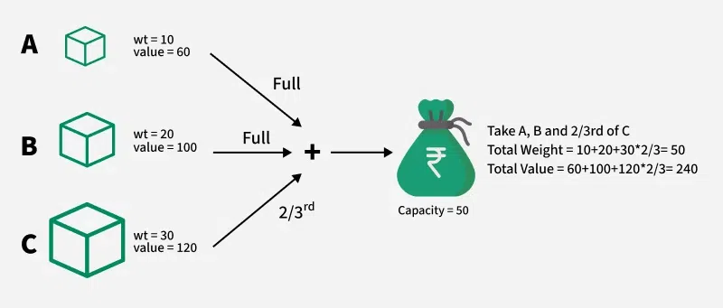
This looks promising. It seems the ability to take fractions prevents the "foreclosed future option" problem. By taking the highest-density item, we are always making the most efficient use of every kilogram of capacity. Intuitively, this feels correct. But to be sure, we need a more robust justification than just our gut feeling. This is where the exchange argument comes in.

The Exchange Argument for Fractional Knapsack

The exchange argument is a way to prove that our greedy choice is "safe" at every step. The logic goes like this: Assume there is some optimal solution that is different from our greedy solution. We will show that we can transform that optimal solution into our greedy one without decreasing its total value, thus proving that the greedy solution is itself optimal.

Let's walk through it.

1. Let G be the solution generated by our greedy algorithm (taking items in descending order of value density).
2. Let O be any optimal solution.
3. If G and O are identical, we are done. If not, they must differ in the amount they take of at least one item. Let i be the highest-density item. Our greedy algorithm G takes as much of i as possible.
4. Suppose the optimal solution O takes less of item i than G does. To fill that weight, O must have taken more of some other item j, where j has a lower value density than i.
5. The Exchange: We can modify O to create a new solution, O'. We take a small amount of weight (say, x kg) from item j out of the knapsack and replace it with x kg of item i. We can do this because O didn't take the full amount of i that was available.
6. The Result: Since item i has a higher value density than j, replacing x kg of j with x kg of i will increase the total value of the solution (or leave it the same if the densities were equal).
7. By repeating this exchange process, we can transform O step-by-step to match the choices of G, at each step never decreasing the total value. Eventually, we will have transformed O into G, proving that G must be at least as good as any arbitrary optimal solution. Therefore, G is optimal.

This argument confirms that always taking as much as possible of the highest-density item is a safe, and ultimately optimal, strategy for the Fractional Knapsack problem.

The following resource gives a formal summary of the proofs for both optimal substructure and the greedy-choice property for the Fractional Knapsack problem. Focus on the Greedy-Choice Property part, as it's a concise version of the exchange argument we just discussed.

Conclusion

In this lesson, we put our greedy algorithm validation skills to the test. We saw that the same problem with a seemingly small change in rules—divisible vs. indivisible items—can completely change whether a greedy strategy is effective.

Here are the key takeaways:

• Always test a greedy rule with counterexamples first. This is the quickest way to find flaws. If you can find even one input where the greedy choice leads to a suboptimal result, the algorithm is incorrect. We did this for three different greedy rules on the 0-1 Knapsack problem.
• The 0-1 Knapsack is a classic case where greedy fails. A locally optimal choice can lock you out of a better global solution.
• The Fractional Knapsack is a classic case where greedy succeeds. The ability to take fractions ensures that prioritizing by value density is always the right move.
• Use an exchange argument to prove a greedy strategy is correct. The core logic is to show that you can swap your greedy choice into any supposed optimal solution without making it worse, thereby proving your greedy solution is one of the optimal solutions.

In our next lesson, we will continue exploring greedy patterns by looking at problems involving intervals. We'll see how sorting by a particular attribute, like we did with finish times and value densities, is a recurring theme in designing correct greedy algorithms.