Identifying Greedy Choices and Safety Properties

Welcome to the ninth module of our course! We've spent a good deal of time building a solid foundation with fundamental algorithms and data structures. Now, we'll start exploring higher-level problem-solving paradigms, which are powerful tools for your interview toolkit. This module is all about Greedy Algorithms.

In this first lesson, we'll dive into the core philosophy of this approach. You'll learn what it means for an algorithm to be "greedy" by focusing on its central component: the local choice it makes at every step. More importantly, we'll tackle the most critical question: how can you determine if that immediate, seemingly best choice is actually "safe" and won't lead you to a dead end? By the end of our session, you'll be able to identify the greedy choice in a potential solution and describe the property that must hold for it to be correct.

What is a Greedy Algorithm?

At its heart, a greedy algorithm is an approach that builds up a solution piece by piece, always choosing the option that offers the most obvious and immediate benefit. It makes a locally optimal choice at each stage with the hope of finding a globally optimal solution.

Imagine you need to give someone change for 67 cents using standard US coins (1, 5, 10, 25 cents), and you want to use the fewest coins possible. A natural, greedy approach would be:

1. Take the largest coin that isn't more than the remaining amount (a quarter, 25c). Amount remaining: 42c.
2. Take another quarter. Amount remaining: 17c.
3. A quarter is too big. Take a dime (10c). Amount remaining: 7c.
4. A dime is too big. Take a nickel (5c). Amount remaining: 2c.
5. Take a penny (1c). Amount remaining: 1c.
6. Take another penny. Amount remaining: 0.

This works perfectly. The locally optimal choice ("always take the largest possible coin") leads to the globally optimal solution (the minimum number of coins). This intuitive idea is the basis for all greedy algorithms.

To get a more formal handle on this, the following article provides a concise definition of the greedy approach and its key characteristics.

The article you just read mentions two crucial properties:

• Greedy Choice Property: This is the big one. It means that a globally optimal solution can be arrived at by making a sequence of locally optimal choices. In other words, making the "best" choice right now doesn't prevent you from reaching the best overall outcome. You never need to go back and undo a choice.
• Optimal Substructure: This means that an optimal solution to the problem contains within it optimal solutions to subproblems. In our coin example, after giving a 25c coin for a 67c total, the remaining problem (making change for 42c) is just a smaller version of the same problem, and its optimal solution is part of the overall optimal solution.

This second property is also shared by another powerful technique called Dynamic Programming (DP), which we'll cover later. The key difference, as noted in the article from DSA Lab, is that a greedy algorithm commits to its choice, while DP would explore all possible choices to find the best one. When a greedy approach works, it's almost always simpler and faster.

The Critical Question: Is the Greedy Choice Safe?

The simplicity of greedy algorithms can be deceptive. The "greedy" strategy of always picking the largest coin feels right, but does it always work? This is the most important question to ask when designing or evaluating a greedy algorithm.

Let's modify the coin problem slightly. Imagine a currency system with coins worth {1, 3, 4}. You need to make change for 6.

What does our greedy algorithm do?

1. It takes the largest coin available: 4.
2. The remaining amount is 2. The next largest coin it can take is 1.
3. The remaining amount is 1. It takes another 1.
   The greedy solution is {4, 1, 1}, which is 3 coins.

However, a better solution exists: {3, 3}, which is only 2 coins.

In this case, the locally optimal choice (taking the 4) was a mistake. It led to a suboptimal global solution. The greedy choice was not "safe." This failure is a classic counterexample that shows the greedy approach for coin changing doesn't work for all coin systems.

The article we looked at earlier highlights this exact scenario.

So, if we can't just trust our intuition, how do we determine if a greedy choice is safe? We need a more structured way to reason about it. There are two main techniques:

1. Refutation by Counterexample: Try to find a small, specific input where the greedy choice leads to a worse result than some other choice. This is exactly what we did with the {1, 3, 4} coin system. If you can find even one counterexample, the greedy strategy is proven incorrect.
2. Validation by Exchange Argument: This is an intuitive but powerful way to argue that a greedy choice is safe. You don't need a formal mathematical proof, but you need to be able to explain the logic.

Let's explore this with a famous problem where a greedy strategy works beautifully: Interval Scheduling.

Case Study: The Interval Scheduling Problem

Imagine you have a single resource, like a meeting room, and a list of requested meetings, each with a start and end time. Your goal is to schedule the maximum possible number of non-overlapping meetings.

Here is a set of proposed meetings (or intervals):

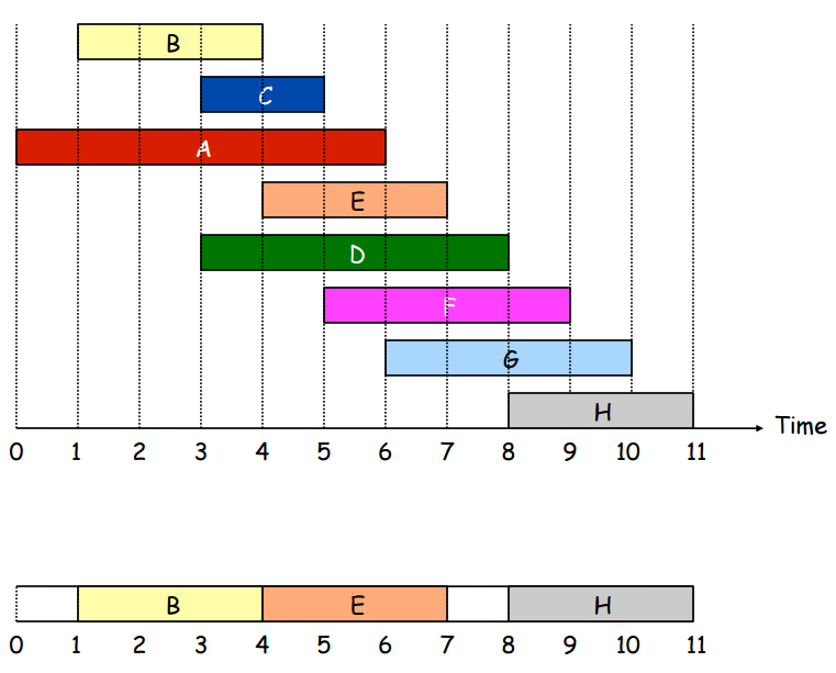
What would a greedy strategy look like here? We need to decide what to be "greedy" about. Here are a few candidate greedy rules:

1. Choose the earliest start time: Pick the interval that starts first. This seems plausible—it gets a meeting on the books right away.
2. Choose the shortest duration: Pick the interval that takes up the least amount of time. This also seems plausible, as it might leave more room for others.
3. Choose the earliest finish time: Pick the interval that finishes first, regardless of when it started.

Which of these is a "safe" move? Let's test them.

• Earliest Start Time: Look at the chart. Interval A starts earliest (at time 0). If we pick A, it occupies the room until time 6. This prevents us from picking B, C, D, and E. We can then only pick G or H. A solution might be {A, G}. That's only 2 meetings. The solution {B, E, H} has 3 meetings. So, "earliest start time" is not a safe greedy choice. We found a counterexample.
• Shortest Duration: Interval C has the shortest duration (2 units). If we pick C, we can't pick A, B, D, or E. We could then pick G or H. A solution could be {C, G}. Again, only 2 meetings. We have a counterexample.
• Earliest Finish Time: Interval B finishes earliest (at time 4). If we pick B, we eliminate A and C as possibilities. The remaining available intervals are D, E, F, G, H. Of these, E finishes earliest (at time 7). We pick E. This eliminates D, F, and G. The only remaining interval is H, which doesn't conflict. We pick H. Our solution is {B, E, H}, which contains 3 meetings. This matches the optimal solution shown in the image.

It seems that "earliest finish time" is the correct greedy choice. But why? The intuition is that by finishing as early as possible, we leave the resource available for the maximum amount of time for other potential activities. This choice keeps our future options as open as possible.

The Exchange Argument: Justifying the Safe Choice

We can formalize this intuition with an exchange argument. Here's the logic:

Let's say Greedy is the solution our "earliest finish time" algorithm produces. Let Optimal be any true optimal solution. We want to show that Greedy is just as good as Optimal (i.e., it contains the same number of intervals).

1. Compare the first interval in Greedy (g_1) and Optimal (o_1). Our greedy rule picks the interval with the absolute earliest finish time. So, by definition, g_1 must finish at or before o_1 finishes.

2. If g_1 is the same as o_1, great. They match. We move on to the next interval.

3. If g_1 is different from o_1, we can "exchange" o_1 for g_1 in the Optimal solution. Can we do this? Yes. Since g_1 finishes earlier than o_1, it cannot possibly conflict with the second interval in the Optimal solution (o_2), because o_1 didn't conflict with o_2. By swapping o_1 for g_1, we create a new solution Optimal' that is still valid and has the same number of intervals.

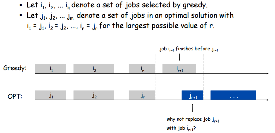
We can repeat this argument for every interval. We can transform any Optimal solution, step by step, into the Greedy solution without ever decreasing the number of intervals. Therefore, the Greedy solution must contain the same number of intervals as any Optimal solution, which means it is itself optimal.

This line of reasoning is the heart of validating a greedy algorithm. The following video provides an excellent, detailed walkthrough of this exact proof. While you don't need to memorize the formal steps, focus on understanding the core logic of the exchange.

Summary and Key Takeaways

Thinking greedily is a powerful problem-solving technique, but it requires careful validation. The "greedy" part is easy—the hard part is proving your greed is justified.

Here's the mental checklist to use when you suspect a problem might have a greedy solution:

1. Identify a Greedy Choice: Propose a rule for making a locally optimal choice. What are you prioritizing? (e.g., largest value, smallest weight, earliest finish time).
2. Look for Counterexamples: Actively try to prove your rule wrong with small, tricky inputs. If you find one, your strategy is flawed. This is often the fastest way to eliminate incorrect greedy approaches.
3. Formulate an Exchange Argument: If you can't find a counterexample, try to articulate why the choice is safe. The core idea is usually that your greedy choice "leaves maximum room" or "uses minimum resources" for the rest of the problem, and can be swapped into any optimal solution without penalty.

In our next lesson, we will continue practicing this skill. We will look at another problem, propose a few different greedy strategies, and use counterexamples and exchange arguments to validate or refute them.