Double DQN for Overestimation Reduction

Hello! Welcome back to our journey into Deep Reinforcement Learning.

In our last lesson, we built a Deep Q-Network (DQN), combining Q-learning with neural networks, experience replay, and a target network to create a stable and powerful learning agent. We saw how the target network, by providing a stable Q-value estimate for the next state, helped prevent the training process from chasing a moving target.

However, the standard DQN algorithm has a subtle but significant flaw: it tends to be overly optimistic. This lesson focuses on addressing that flaw.

Today's learning outcome is to implement Double DQN to reduce overestimation bias. We'll first understand why DQN systematically overestimates Q-values and then explore the elegant solution provided by Double DQN, which involves a minor but crucial change to the target calculation.

Recap: The DQN Target

Recall the TD target calculation from our previous lesson:

y_{t}^{DQN} = r_{t + 1} + γ a^{'} max Q (S_{t + 1}, a^{'}; θ^{-})

Here, we use the target network ( $Q$ with parameters $θ^{-}$ ) to both select the best action in the next state ( $max_{a^{'}}$ ) and evaluate the value of that action. This coupling of selection and evaluation is the source of the problem.

1. The Problem: Q-Value Overestimation

Why is taking the maximum a problem? Imagine your Q-network is still learning, so its estimates are noisy. Some Q-values will be randomly higher than they should be, and others will be lower. When you take the max over these noisy values, you are more likely to pick an action whose value has been overestimated. This leads to a persistent positive bias in your Q-value estimates, causing the agent to be "overly optimistic" about certain actions. This can slow down learning and lead to suboptimal policies.

To build your intuition on this, let's watch a short video that explains the problem using a simple analogy.

Double DQN (DDQN) Explained & Implemented | DQN PyTorch Beginners Tutorial #10

The 'Johnny Code' channel provides a great analogy using a modified Flappy Bird game to explain how overestimation can lead an agent to waste time on suboptimal paths.

Watch the first 3 minutes and 37 seconds of the video. Focus on how the max function can initially mislead the agent into choosing a path that seems good in the short term but is ultimately a dead end.

This overestimation isn't just an experimental quirk; it's a known issue in Q-learning, which is exacerbated when using flexible function approximators like neural networks.

This image provides a great visualization of the effect. In a simple gridworld, standard Q-Learning overestimates the values of many states compared to the more accurate estimates from Double Q-Learning.

Overestimation Bias in Q-Learning vs Double Q-Learning — This image compares Q-value estimates in a gridworld. Standard Q-Learning (left) shows several overestimated values (in red). Double Q-Learning (right) mitigates this bias, leading to more accurate, and generally lower, Q-values.

2. The Solution: Decoupling Selection and Evaluation

The core idea of Double DQN is to break the dependency where the same network both chooses the best action and evaluates its worth. Instead, we decouple these two steps:

Action Selection: Use the online network (with weights $θ_{t}$ ) to determine which action is best for the next state, $S_{t + 1}$ . $a^{*} = a^{'} argmax Q (S_{t + 1}, a^{'}; θ_{t})$
Action Evaluation: Use the target network (with weights $θ_{t}^{-}$ ) to estimate the Q-value of that specific action $a^{*}$ .

This changes our target calculation.

DQN Target:

Y_{t}^{DQN} = R_{t + 1} + γ Selection and evaluation by target network Q (S_{t + 1}, a^{'} argmax Q (S_{t + 1}, a^{'}; θ_{t}^{-}); θ_{t}^{-})

Double DQN Target:

Y_{t}^{DoubleDQN} = R_{t + 1} + γ Selection by online network Evaluation by target network Q (S_{t + 1}, a^{'} argmax Q (S_{t + 1}, a^{'}; θ_{t}), θ_{t}^{-})

In essence, the online network proposes what it thinks is the best next move, and the more stable target network gives a second, less biased opinion on the value of that move. Since the errors in the two networks are unlikely to be correlated, it's less likely that we'll overestimate the value.

The following article and video provide excellent explanations of this change.

Improving the DQN algorithm using Double Q-Learning

The article 'Improving the DQN algorithm using Double Q-Learning' provides the mathematical formulas and a concise explanation of this decoupling.

Read the section 'Implementing the Double DQN algorithm'. Focus on the two mathematical formulas provided for the DQN and Double DQN targets. See how the arguments inside the outer Q-function change.

Now, let's watch a visual walkthrough of this two-step process.

Double DQN (DDQN) Explained & Implemented | DQN PyTorch Beginners Tutorial #10

Let's return to the 'Johnny Code' video. This segment provides a clear whiteboard explanation of how the online and target networks collaborate to calculate the DDQN target.

Watch from 05:47 to 08:58. Pay close attention to the two-step process he describes: Using the policy network (online network) to get the best action index. Using that index to get the Q-value from the target network.

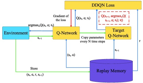
This diagram summarizes the flow of information in a DDQN architecture.

Double Deep Q-Network (DDQN) Architecture — This diagram illustrates the DDQN architecture. The key difference from DQN is in how the target is calculated. The Q-Network (online network) selects the best action for the next state, and the Target Q-Network provides the value for that selected action, which is then used to compute the DDQN loss.

Test your understanding!

An agent is in state $S_{t}$ and takes action $A_{t}$ , receiving reward $R_{t + 1}$ and moving to state $S_{t + 1}$ . Let $γ = 0.9$ .

The online network's Q-values for the next state $S_{t + 1}$ are:

$Q (S_{t + 1}, action_{0}; θ_{t}) = 1.5$
$Q (S_{t + 1}, action_{1}; θ_{t}) = 1.8$

The target network's Q-values for the next state $S_{t + 1}$ are:

$Q (S_{t + 1}, action_{0}; θ_{t}^{-}) = 1.4$
$Q (S_{t + 1}, action_{1}; θ_{t}^{-}) = 1.6$

What is the DDQN target value $Y_{t}^{DoubleDQN}$ ?
For comparison, what would the DQN target value $Y_{t}^{DQN}$ have been?

Show answer

DDQN Target Calculation:
- Step 1 (Selection): Use the online network to find the best action. The max Q-value is 1.8, corresponding to $action_{1}$ . So, $a^{*} = action_{1}$ .
- Step 2 (Evaluation): Use the target network to get the value of $a^{*}$ . The Q-value for $action_{1}$ in the target network is 1.6.
- Final Target: $Y_{t}^{DoubleDQN} = R_{t + 1} + γ \times 1.6 = R_{t + 1} + 0.9 \times 1.6 = R_{t + 1} + 1.44$ .
DQN Target Calculation:
- Use the target network for both selection and evaluation. The max Q-value in the target network is 1.6.
- Final Target: $Y_{t}^{DQN} = R_{t + 1} + γ \times 1.6 = R_{t + 1} + 0.9 \times 1.6 = R_{t + 1} + 1.44$ .
Note: In this specific case, both targets are the same because the best action was the same for both networks. However, if the online network had estimated $Q (S_{t + 1}, action_{0}; θ_{t}) = 2.0$ , DDQN would have selected $action_{0}$ and evaluated it with the target network's value of 1.4, resulting in a lower target than DQN's.

3. Implementing Double DQN

The best part about Double DQN is its simplicity. You don't need a new network or a complex new algorithm. You just need to modify a single line of code in your existing DQN optimize (or learn) function.

This short clip shows how trivially you can add a check for DDQN and change the target calculation logic.

Double DQN (DDQN) Explained & Implemented | DQN PyTorch Beginners Tutorial #10

Here's the code change from the 'Johnny Code' tutorial. It's a simple if/else block that switches between the DQN and DDQN target calculations.

Watch from 09:10 to 10:22. Notice how the DDQN implementation first gets the Q-values for the next state from the online network (self.policy_net), finds the argmax to get the best actions, and then uses these actions to gather the corresponding values from the target network's output.

To see this in the context of a full agent class, we'll look at a more complex implementation. The following video implements "Dueling Double DQN," which combines two separate improvements. For now, ignore the "Dueling" aspect of the network architecture; we are only interested in the learn function, which contains the pure Double DQN update rule.

Dueling Double Deep Q Learning is Easy in PyTorch

This video by 'Machine Learning with Phil' shows the DDQN update rule within a complete agent's learn method. We'll focus only on the relevant lines for the DDQN target calculation.

Watch from 33:35 to 38:50. This section is quite dense, so focus on this specific sequence of operations: (around 35:00) Pass new_states through both q_eval (online) and q_next (target) networks. (around 35:30) Calculate max_actions by taking the argmax of the online network's output (q_eval). This is the action selection step. (around 38:00) The final target q_target is calculated by adding the reward to gamma multiplied by the target network's output (q_next), but indexed at the max_actions determined by the online network. This is the action evaluation step. The rest of the code is related to the Dueling architecture, which you can disregard for this lesson.

The implementation, once you locate it, is a direct translation of the DDQN formula. First, you get the next-state Q-values from both networks. Then you use the online network's values to find the indices of the best actions. Finally, you use those indices to select the Q-values from the target network's output to form your final target.

Summary: DQN vs. DDQN

This table provides a final, clear comparison between the two algorithms.

Double Deep Q-Network (DDQN)

The 'Emergent Mind' page on DDQN has an excellent summary table that puts everything side-by-side.

Review the 'Summary Table: Core Components and Comparisons'. This is a perfect way to solidify your understanding of the key differences.

Conclusion

In this lesson, we tackled a key weakness of the standard DQN algorithm. By understanding and fixing the overestimation bias, you've taken another step toward building more robust and effective RL agents.

Key Takeaways:

DQN Overestimation: The max operator in the DQN target calculation causes a systematic overestimation of Q-values, which can lead to suboptimal policies.
Decoupled Selection & Evaluation: Double DQN resolves this by using the online network to select the best action for the next state and the target network to evaluate the value of that chosen action.
The DDQN Target: The new target is $Y_{t}^{DoubleDQN} = R_{t + 1} + γ Q (S_{t + 1}, a^{'} argmax Q (S_{t + 1}, a^{'}; θ_{t}), θ_{t}^{-})$ .
Minimal Implementation Change: Implementing DDQN requires only a small modification to the target calculation logic within an existing DQN codebase.

Preview of the Next Lesson:

So far, our agents have focused on learning the values of state-action pairs (Q-values). We then derive a policy from these values (e.g., by taking the argmax). The next lesson introduces a fundamentally different family of algorithms: Policy Gradient methods. Instead of learning a value function, we will directly learn and optimize the policy itself. Our first algorithm in this new domain will be REINFORCE.