Implementing REINFORCE

Hello! Welcome to the next lesson in our Deep Reinforcement Learning module.

In our previous lessons, we explored value-based methods like DQN and Double DQN. These algorithms learn a value function (Q-values) and then use it to implicitly define a policy, for example, by always choosing the action with the highest Q-value. This approach has been incredibly successful, but it's not the only way to solve RL problems.

Today, we shift our perspective to a different class of algorithms: policy gradient methods. Instead of learning values and inferring a policy, we will directly learn the parameters of the policy itself.

Our learning outcome for this lesson is to implement the REINFORCE algorithm, which is the most fundamental policy gradient method. We will explore its theoretical underpinnings, understand its practical implementation, and identify its core limitations, which will set the stage for our next topic.

1. From Value-Based to Policy-Based RL

In value-based methods, our policy is often deterministic (e.g., $\pi (s)=\arg {\max }_{a}Q(s,a)$). Policy-based methods, however, directly parameterize the policy ${\pi }_{\theta }(a|s)$, which can be a neural network that outputs a probability distribution over actions given a state.

Our goal is to find the parameters $\theta$ that maximize an objective function, typically the expected total reward. We achieve this using gradient ascent.

The key advantages of this direct approach are:

• Continuous Action Spaces: It can naturally handle continuous action spaces, where outputting a Q-value for every possible action is intractable.
• Stochastic Policies: It can learn truly stochastic policies, which can be optimal in environments where a deterministic policy might fail (e.g., in a game of rock-paper-scissors).

Let's begin with a video that contrasts policy gradient methods with the value-based methods we've already covered.

2. The Policy Gradient Theorem

The core challenge in policy gradient methods is computing the gradient of the objective function $J(\theta )$ with respect to the policy parameters $\theta$. The objective function depends on the state distribution induced by the policy, and this dependency is complex and usually unknown.

Fortunately, the Policy Gradient Theorem provides a way to compute this gradient without needing to differentiate the state distribution. It gives us an expression for the gradient that we can estimate from experience.

This expression can be rewritten using a common identity known as the log-derivative trick: ${\nabla }_{\theta }{\pi }_{\theta }(a|s)={\pi }_{\theta }(a|s){\nabla }_{\theta }\log {\pi }_{\theta }(a|s)$. Substituting this into the theorem and rearranging gives a very useful form expressed as an expectation:

$${\nabla }_{\theta }J(\theta )={\mathbb{E}}_{{\pi }_{\theta }}[Q^{\pi }(s,a){\nabla }_{\theta }\log {\pi }_{\theta }(a|s)]$$

This equation tells us that to perform gradient ascent, we should nudge the parameters $\theta$ in the direction of ${\nabla }_{\theta }\log {\pi }_{\theta }(a|s)$ (which increases the probability of action $a$ in state $s$), and the size of this nudge should be proportional to the action-value $Q^{\pi }(s,a)$. In other words: if an action leads to a good outcome, increase its probability.

3. REINFORCE: A Monte Carlo Policy Gradient Algorithm

The REINFORCE algorithm, also known as Monte-Carlo Policy Gradient, applies this theorem in the simplest way possible. It recognizes that the true action-value, $Q^{\pi }(S_t,A_t)$, is the expected return from that point onward. A simple, unbiased estimate for this expected return is the actual, observed return from a single trajectory, which we'll call $G_t$.

So, we can replace $Q^{\pi }(s,a)$ with the Monte Carlo return $G_t$. The gradient update becomes:

$${\nabla }_{\theta }J(\theta )={\mathbb{E}}_{{\pi }_{\theta }}[G_t{\nabla }_{\theta }\log {\pi }_{\theta }(A_t|S_t)]$$

This leads to the REINFORCE algorithm:

1. Generate an episode: Using the current policy ${\pi }_{\theta }$, run a full episode from start to finish, collecting states, actions, and rewards: $(s_0,a_0,r_1),(s_1,a_1,r_2),\dots ,(s_{T-1},a_{T-1},r_T)$.
2. Calculate returns: For each time step $t$ in the episode, calculate the discounted return $G_t={\sum }_{k=t}^{T-1}{\gamma }^{k-t}{r}_{k+1}$. This is the "reward-to-go".
3. Update the policy: Update the policy parameters using gradient ascent. The update for a single step $t$ is proportional to $G_t{\nabla }_{\theta }\log {\pi }_{\theta }(A_t|S_t)$.

Let's watch a video that walks through these steps and explains how to implement them.

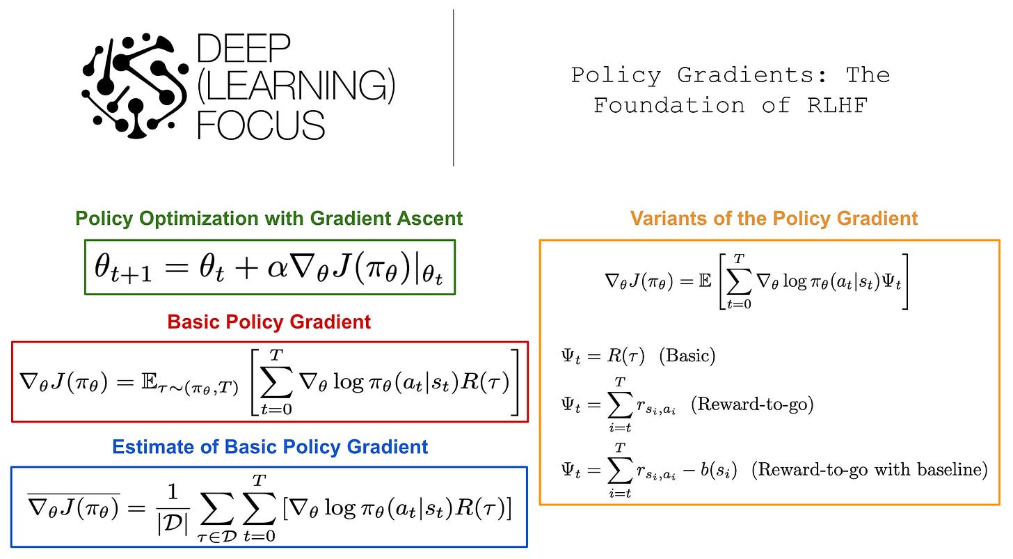
The image below, from the article "REINFORCE: Easy Online RL for LLMs," summarizes the key formulas for policy gradients, including the basic form used by REINFORCE and a variant with a baseline, which we will discuss shortly.

Test your understanding!

An agent is using REINFORCE. It completes a short episode of 3 steps:

• Step 0: takes action $a_0$ in state $s_0$, gets reward $r_1=-1$.
• Step 1: takes action $a_1$ in state $s_1$, gets reward $r_2=+3$.
• Step 2: takes action $a_2$ in state $s_2$, gets reward $r_3=-5$, and the episode ends.

Assume the discount factor $\gamma =0.9$ and the learning rate $\alpha =0.01$.

1. What is the return $G_t$ for each time step $t=0,1,2$?
2. Which action's log-probability will be most strongly increased by the update? Which will be most strongly decreased (or least increased)?

Show answer

1. Calculating Returns (Reward-to-go):

   • $G_2=r_3=-5$
   • $G_1=r_2+\gamma r_3=3+0.9\times (-5)=3-4.5=-1.5$
   • $G_0=r_1+\gamma r_2+{\gamma }^2{r}_3=-1+0.9\times 3+0.81\times (-5)=-1+2.7-4.05=-2.35$

2. Update Direction: The update for each action is proportional to its return $G_t$.

   • Action $a_0$ has a return of -2.35.
   • Action $a_1$ has a return of -1.5.
   • Action $a_2$ has a return of -5.

   Since all returns are negative, the algorithm will try to decrease the probability of all three actions. However, the action with the least negative return ($a_1$) will be decreased the least. The action with the most negative return ($a_2$) will be decreased the most. Therefore, relative to the others, $a_1$ is the "best" action in this trajectory and will be reinforced the most (or punished the least).

4. Implementation in PyTorch

Now, let's translate the algorithm into code. The implementation follows the steps we just outlined.

Here is a conceptual Python/PyTorch implementation that captures the essence of the algorithm for a single training iteration (one episode):

import torch
import torch.nn as nn
from torch.distributions import Categorical

# Assume 'env', 'policy_net', and 'optimizer' are defined
# policy_net is an nn.Module that outputs logits for actions

# --- 1. Generate an episode ---
saved_log_probs = []
rewards = []
state, _ = env.reset()
done = False

while not done:
    # Get action probabilities from the policy network
    state_tensor = torch.from_numpy(state).float().unsqueeze(0)
    action_logits = policy_net(state_tensor)
    action_dist = Categorical(logits=action_logits)
    
    # Sample an action and save its log probability
    action = action_dist.sample()
    saved_log_probs.append(action_dist.log_prob(action))
    
    # Take the action in the environment
    state, reward, terminated, truncated, _ = env.step(action.item())
    rewards.append(reward)
    done = terminated or truncated

# --- 2. Calculate returns and assemble loss ---
returns = []
discounted_return = 0
# Iterate through rewards in reverse order
for r in rewards[::-1]:
    discounted_return = r + gamma * discounted_return
    returns.insert(0, discounted_return) # Prepend to keep order

returns = torch.tensor(returns)
# Standardize returns for better performance (a simple form of baseline)
returns = (returns - returns.mean()) / (returns.std() + 1e-9)

policy_loss = []
for log_prob, R in zip(saved_log_probs, returns):
    # The loss for one step is -log_prob * Return
    # We want to maximize log_prob * R, so we minimize -(log_prob * R)
    policy_loss.append(-log_prob * R)

# --- 3. Update the policy ---
optimizer.zero_grad()
loss = torch.cat(policy_loss).sum() # Sum losses over the episode
loss.backward()
optimizer.step()

5. The Problem with REINFORCE: High Variance

REINFORCE works, but it has a major drawback: high variance. The return $G_t$ from a single trajectory can be very noisy. A good action might be part of an overall unlucky trajectory, receiving a negative return and being discouraged. A bad action might be part of a lucky trajectory and be reinforced. This makes learning unstable and slow.

The solution is to subtract a baseline $b(s_t)$ from the return. The update rule becomes proportional to $(G_t-b(s_t)){\nabla }_{\theta }\log {\pi }_{\theta }(A_t|S_t)$.

A good baseline should only depend on the state $s_t$, not the action $a_t$. This ensures the update remains unbiased. A common and effective baseline is the state-value function, $V(s_t)$. The term $G_t-V(s_t)$ is an estimate of the advantage function $A(s_t,a_t)$, which measures how much better taking action $a_t$ was than the average action from state $s_t$.

• If $A(s_t,a_t)>0$, the action was better than average; increase its probability.
• If $A(s_t,a_t)<0$, the action was worse than average; decrease its probability.

This is a much more stable learning signal.

Notice in the code snippet above, we already included a simple baseline: standardizing the returns for the batch (returns = (returns - returns.mean()) / (returns.std())). This centers the returns around zero, ensuring some actions get positive reinforcement and others get negative, which is a simple but effective way to reduce variance.

Conclusion

In this lesson, we made the leap from value-based to policy-based reinforcement learning. We explored the theoretical foundation of policy gradient methods and implemented REINFORCE, the simplest algorithm in this family.

Key Takeaways:

• Policy Gradient Methods directly optimize a parameterized policy ${\pi }_{\theta }(a|s)$ via gradient ascent on the expected reward.
• The Policy Gradient Theorem provides a way to compute the policy gradient without differentiating the environment dynamics.
• REINFORCE is a Monte Carlo algorithm that uses the observed return $G_t$ from an episode as an unbiased estimate for $Q^{\pi }(S_t,A_t)$.
• The update rule for REINFORCE pushes up the log-probability of an action in proportion to the return that followed it.
• REINFORCE suffers from high variance, which makes training unstable. This can be mitigated by subtracting a baseline, such as the state-value function $V(s)$, from the return.

Preview of the Next Lesson:

The idea of using the value function $V(s)$ as a baseline is powerful. But how do we get $V(s)$ if we are only learning a policy? The answer is: we learn it! This leads directly to our next topic: Actor-Critic methods. We will build an agent with two components: an Actor (the policy) that decides what to do, and a Critic (the value function) that evaluates how good those decisions are.