Implementing Deep Q-Networks (DQN)

Hello! Welcome to the first lesson in our module on Deep Reinforcement Learning.

In our previous module, we established the foundations of RL, culminating in the distinction between on-policy and off-policy learning. We saw that off-policy methods like Q-learning are highly sample-efficient because they can learn from a buffer of past experiences—a technique called experience replay. However, all the methods we've used so far relied on Q-tables, which are simply not feasible for environments with large or continuous state spaces.

Today, we bridge that gap. We'll combine the power of deep neural networks with Q-learning to create an agent that can learn in much more complex environments.

This lesson directly addresses the learning outcome: Implement a Deep Q-Network (DQN) with experience replay and a target network. We will unpack the theory behind DQN and then walk through a full implementation in PyTorch.

1. From Tables to Networks: The Need for Function Approximation

The core limitation of tabular methods is the "curse of dimensionality." Imagine an environment like an Atari game where the state is represented by the screen's pixels. An 84x84 pixel grayscale image has $256^{7056}$ possible states. A Q-table to store a value for each state-action pair would be astronomically large and impossible to store, let alone fill with meaningful values.

The solution is to use a function approximator. Instead of a table, we use a parameterized function to estimate the Q-values. Given your background in machine learning, you'll immediately recognize that neural networks are perfect for this role.

This leads to the central idea of a Deep Q-Network: we use a neural network that takes a state $s$ as input and outputs a vector of Q-values, one for each possible action $a$. We can denote this as $Q(s,a;\theta )$, where $\theta$ represents the network's weights.

Training this network becomes a regression problem: we want to adjust the weights $\theta$ so that the network's output $Q(s,a;\theta )$ gets closer to the "true" optimal Q-value. However, simply plugging a neural network into the Q-learning update rule leads to instability. The breakthrough of DQN came from two key innovations that stabilize the training process.

2. The Core Components of DQN

The original DeepMind paper, which demonstrated superhuman performance on Atari games, introduced two crucial techniques on top of the basic Q-network: Experience Replay and a Target Network.

Let's break down each component in more detail.

A. Experience Replay

As we briefly touched upon in the last lesson, training a neural network on highly correlated data—like consecutive frames from a game—is a recipe for disaster. The model can overfit to recent experiences and forget what it learned before.

Experience Replay solves this by creating a large buffer (often implemented as a deque in Python) that stores transitions the agent observes: $(s_t,a_t,r_{t+1},s_{t+1})$. To update the network, we don't use the most recent transition. Instead, we sample a random mini-batch of transitions from this buffer.

This has two major benefits:

1. Breaking Correlations: Random sampling breaks the temporal correlations in the data, making the training updates more stable and independent, similar to the i.i.d. assumption in supervised learning.
2. Data Efficiency: Each experience can be reused multiple times in different training batches, allowing the agent to learn more from each interaction with the environment.

B. The Target Network

The second source of instability comes from the Q-learning update rule itself. Recall the temporal difference (TD) target from Q-learning:

$$y_t=R_{t+1}+\gamma \underset{a^{\prime }}{\max }Q(S_{t+1},a^{\prime };\theta )$$

We are trying to update our network's prediction, $Q(S_t,A_t;\theta )$, to be closer to this target, $y_t$. The problem is that the same network weights $\theta$ are used to compute both the prediction and the target. This is like trying to hit a target that moves every time you adjust your aim. This "chasing a moving target" problem can cause oscillations and prevent the training from converging.

The solution is to use two separate networks:

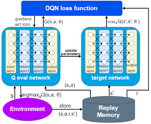
1. Policy Network ($Q(s,a;\theta )$): This is the main network that we are actively training. It is used to select actions (during exploitation) and to calculate the Q-value for the current state.
2. Target Network ($Q(s,a;{\theta }^{-})$): This is a copy of the policy network. Its weights ${\theta }^{-}$ are frozen for a period of time. This network is used to calculate the value of the next state for the TD target, providing a stable, consistent target for the policy network to learn towards.

$$y_t=R_{t+1}+\gamma \underset{a^{\prime }}{\max }Q(S_{t+1},a^{\prime };{\theta }^{-})$$

The weights of the target network (${\theta }^{-}$) are periodically updated with the weights from the policy network ($\theta$). This can be a "hard" update (a direct copy every C steps) or a "soft" update (a slow, weighted average).

This diagram provides a great visual summary of how all the components interact.

3. The DQN Algorithm and Implementation

With these concepts in place, we can now walk through a full implementation. We'll use the FrozenLake environment from the gymnasium library, which is simple enough to let us focus on the DQN mechanics.

The following video from the "Johnny Code" channel provides an exceptionally clear, step-by-step walkthrough of building a DQN in PyTorch. We will watch it in segments to understand each part of the implementation.

Now, let's dive into the code.

Step 1: The DQN and ReplayMemory Classes

The first two pieces we need are the neural network itself and the class for our experience replay buffer.

For comparison, the official PyTorch DQN tutorial provides a similar implementation. Note that it uses a namedtuple for the Transition, which is a clean way to organize the stored experience.

Step 2: The Training Loop

This is where everything comes together. The main training function will initialize the environment, networks, and replay buffer. Then, it will loop through episodes, and within each episode, it will:

1. Select an action using an $ϵ$-greedy policy.
2. Execute the action and observe the outcome.
3. Store the transition in the replay buffer.
4. Sample a mini-batch from the buffer and perform an optimization step.
5. Periodically update the target network.

Test your understanding!

In the DQN algorithm, we use two networks: the policy network and the target network.

1. Why do we need the target network? What would happen if we used the policy network to calculate the TD target $y_t$?
2. In the optimize function, we pass next_states through the target network but current_states through the policy network. Why don't we use the target network for both?

Show answer

1. The target network is needed for stability. If we used the policy network to calculate the TD target, the target value would change at every single training step. This makes the learning process unstable, as the policy network would be "chasing a moving target." By using a target network that is updated only periodically, we provide a stable, consistent target for the policy network to converge towards.

2. The goal of the optimization step is to update the policy network. We want to adjust its weights $\theta$ to make its prediction $Q(s,a;\theta )$ for the current state more accurate. The target network's role is only to provide a stable value for the next state to compute the TD target. We don't want to update the target network during this step (its gradients are detached), and we're not trying to select actions with it—we're just using it as a stable value function approximator for $V(s^{\prime })$.

4. A More Complex Example: Lunar Lander and Soft Updates

The FrozenLake environment has a discrete state space, which we one-hot encode. To see the true power of DQN, let's look at an environment with a continuous state space, LunarLander-v2. Here, the state is a vector of 8 continuous values (position, velocity, angle, etc.).

This also gives us a chance to introduce a common refinement: the soft update. Instead of a hard copy of weights every C steps, we slowly blend the policy network's weights into the target network at every step:
${\theta }^{-}\leftarrow \tau \theta +(1-\tau ){\theta }^{-}$
where $\tau$ is a small hyperparameter (e.g., 0.005). This leads to even more stable training.

Conclusion

Congratulations on completing your first foray into Deep Reinforcement Learning! You've gone from the tabular world of Q-learning to a powerful deep learning-based agent.

Key Takeaways:

• DQN uses a neural network to approximate the Q-function, allowing it to handle large, high-dimensional state spaces.
• Experience Replay is crucial for stabilizing training by storing transitions in a buffer and sampling random mini-batches, which breaks temporal correlations and improves data efficiency.
• A separate Target Network provides stable TD targets, preventing the learning process from becoming unstable due to a "moving target" problem.
• The DQN loss function is typically the Mean Squared Error or Huber Loss between the target Q-value (from the target network) and the predicted Q-value (from the policy network).
• The target network can be updated with a hard copy periodically or with a soft update at each step.

Preview of the Next Lesson:

While DQN is a massive step forward, it has a known flaw: it tends to be overly optimistic and systematically overestimates Q-values. In our next lesson, we will explore why this happens and implement Double DQN, an elegant modification that helps to reduce this overestimation bias and further improve performance.