Implementing Advanced Architectural Patterns

Hello! Welcome back to our exploration of landmark CNN architectures.

Introduction

In our previous lesson, we examined the architectural evolution that pushed neural networks deeper and deeper, culminating in ResNet's elegant solution to the degradation problem. The philosophy was clear: depth was a key driver of performance.

Today, we'll explore a different, parallel philosophy that emerged around the same time: making networks not just deeper, but wider and more computationally efficient. This lesson focuses on the Inception module, the core innovation of the GoogLeNet architecture, which won the 2014 ImageNet challenge. Your learning outcome is to implement advanced architectural patterns like Inception modules.

We will cover:

The motivation behind the Inception module's multi-branch design.
The critical role of 1x1 convolutions as "bottlenecks" to manage computational cost.
How to implement a complete Inception module from scratch in PyTorch.
Advanced factorization techniques used in later Inception versions.

By the end of this lesson, you'll have a strong grasp of this "network-in-network" design pattern and its impact on modern CNNs.

1. The "Wide" Approach: The Inception Module

When designing a CNN layer, a key decision is the choice of kernel size. A 3x3 kernel captures finer, local features, while a 5x5 kernel has a larger receptive field to capture more distributed features. A 1x1 kernel can be used to process features channel-wise. Max-pooling is also a proven feature extraction technique. The question posed by the designers of GoogLeNet was: which one is optimal?

Their answer: why choose? Let's do them all in parallel.

This is the central idea behind the Inception module. Instead of stacking layers sequentially, an Inception module has multiple parallel "branches" with different operations. The outputs of these branches are then concatenated along the channel dimension.

CS 152 NN—17: CNN Architectures: Inception

To understand this core idea, let's start with a conceptual overview from the video 'CS 152 NN—17: CNN Architectures'. It explains the motivation and the initial 'naive' design.

Watch from the beginning to 4:23. This section introduces the 'network within networks' idea and lays out the first version of the Inception module, where 1x1, 3x3, and 5x5 convolutions are applied in parallel to the same input.

This "naive" approach, however, has a major flaw: it's computationally expensive. Applying a 5x5 convolution to an input with a high number of channels (e.g., 256) requires a huge number of parameters and computations. Furthermore, concatenating the outputs would cause the number of channels (the depth of the feature map) to grow uncontrollably at each layer.

2. The Bottleneck: Efficient Dimensionality Reduction

The solution to this computational explosion is the clever use of 1x1 convolutions as a "bottleneck" layer. By placing a 1x1 convolution before the expensive 3x3 and 5x5 convolutions, we can reduce the number of input channels (the depth) that these larger filters have to process.

This has two key benefits:

Drastic Reduction in Parameters: The number of parameters in a convolutional layer depends on (kernel_w * kernel_h * C_in * C_out). By reducing C_in with a cheap 1x1 convolution, the overall parameter count plummets.
Deeper, More Expressive Networks: These 1x1 convolutions are full-fledged neural network layers with their own weights and activation functions. They learn to create compressed, meaningful representations of the input channels before they are passed on.

CS 152 NN—17: CNN Architectures: Inception

The same video provides an excellent, detailed explanation of how these 1x1 bottlenecks work and quantifies the parameter savings.

Watch from 8:36 to 15:38. Pay close attention to the parameter calculations. Seeing the reduction from ~1.2 million parameters to ~330k for a single module makes the benefit of this technique incredibly clear.

The final Inception v1 module combines these ideas.

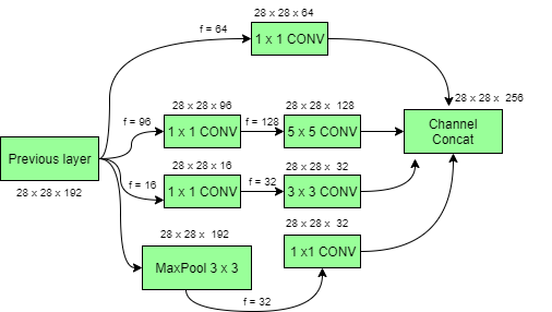
Inception Module Architecture Diagram — The final architecture of an Inception v1 module. Note the 1x1 "bottleneck" convolutions in yellow, which reduce the channel depth before the 3x3 and 5x5 convolutions. The 1x1 convolution after the max-pooling layer serves a similar purpose, ensuring all branches can be concatenated.

The module now consists of four parallel branches:

A simple 1x1 convolution.
A 1x1 convolution (bottleneck) followed by a 3x3 convolution.
A 1x1 convolution (bottleneck) followed by a 5x5 convolution.
A 3x3 max-pooling layer followed by a 1x1 convolution.

The outputs of all four branches, which now have the same spatial dimensions but different channel depths, are concatenated to form the final output of the block.

3. Implementing the Inception Module in PyTorch

Now that we understand the theory, let's translate it into code. Your background in software engineering will be useful here, as building complex architectures like GoogLeNet relies on creating reusable, modular components.

We will follow a from-scratch implementation that clearly shows how each part of the diagram is built.

Pytorch GoogLeNet / InceptionNet implementation from scratch

The video 'Pytorch GoogLeNet / InceptionNet implementation from scratch' by Aladdin Persson provides a clear, step-by-step walkthrough. We'll build the module from the ground up.

Watch from 7:39 to 16:18. The video is structured in two key parts: The ConvBlock (7:39 - 10:22): First, he creates a reusable ConvBlock class containing Conv2d, BatchNorm2d, and ReLU. This is a great programming pattern that keeps the main Inception block code clean. The InceptionBlock (10:22 - 16:18): This is the core implementation. Observe how each of the four branches is defined. branch1 is the 1x1 conv. branch2 and branch3 are nn.Sequential modules containing the bottleneck and the main convolution. branch4 contains the max-pooling and the final 1x1 conv. Finally, see how torch.cat is used in the forward method to combine the outputs.

To solidify your understanding, let's work through an example.

Test your understanding!

Imagine you have an Inception block that takes an input tensor with in_channels=192. The parameters for the branches are set as follows:

out_1x1 = 64 (for the 1x1 branch)
out_3x3 = 128 (for the 3x3 branch, after its bottleneck)
out_5x5 = 32 (for the 5x5 branch, after its bottleneck)
out_1x1pool = 32 (for the max-pool branch)

Question: What will be the number of output channels after the concatenation step in the forward pass?

Show answer

The total number of output channels is the sum of the output channels from each of the four branches.

Total channels = out_1x1 + out_3x3 + out_5x5 + out_1x1pool
Total channels = 64 + 128 + 32 + 32 = 256 channels.

The torch.cat(..., dim=1) operation stacks the tensors along the channel dimension.

To see how these building blocks form a complete network, you can look at the full GoogLeNet implementation. The following text-based resource provides a very clean version.

Build Inception Network from Scratch with Python

The article 'Build Inception Network from Scratch with Python' provides a full PyTorch implementation of GoogLeNet (Inception v1).

Skim through the code in the sections 'Let’s Build Inception v1(GoogLeNet) from scratch:'. Focus on the Inception_block class, which is a great textual reference for what you just saw in the video, and the GoogLeNet class, which shows how these Inception blocks are stacked sequentially, interleaved with max-pooling layers to reduce spatial dimensions.

4. Advanced Patterns: Factorization and Auxiliary Classifiers

The original Inception module was just the beginning. Later versions introduced further refinements to improve efficiency and performance.

Factorizing Convolutions

One key idea was to factorize large convolutions into smaller ones. For example, a 5x5 convolution can be replaced by two stacked 3x3 convolutions. This stack has the same effective receptive field but with fewer parameters and more non-linearities, an idea we first saw with VGG.

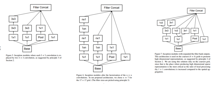
Evolution of Inception Module Architectures — Evolution of Inception modules. **Figure 5** shows a 5x5 convolution being replaced by two 3x3 convolutions. **Figure 6** shows an even more aggressive factorization of an n x n convolution into a 1 x n and n x 1 convolution.

This principle was pushed further by factorizing an n x n convolution into an asymmetric pair of a 1 x n followed by an n x 1 convolution. This is computationally much cheaper and was found to work just as well in practice. These ideas paved the way for even more efficient architectures like MobileNet, which we will study next.

CS 152 NN—17: CNN Architectures: Inception

Let's return to the 'CS 152' video, which explains the logic behind replacing a 5x5 with two 3x3 convolutions.

Watch from 15:38 to 20:57. The video explains why two stacked 3x3 convolutions have the same receptive field as a single 5x5 layer and calculates the reduction in parameters.

Auxiliary Classifiers

GoogLeNet is a very deep network (22 layers). To combat the vanishing gradient problem and ensure that the middle parts of the network receive strong gradient signals during training, the authors added two "auxiliary classifiers". These are small classifiers attached to the output of intermediate Inception blocks. Their loss is added to the main loss of the network (with a smaller weight). During inference, these classifiers are discarded.

CS 152 NN—17: CNN Architectures: Inception

The 'CS 152' video also provides a clear explanation of this training trick.

Watch from 20:57 to 25:29. Understand that this is a technique to improve training for very deep networks by providing additional gradient paths.

Conclusion

You have now explored the innovative architecture of the Inception module, a significant departure from the purely sequential designs of VGG and plain ResNets. By thinking in parallel and focusing on computational efficiency, the designers of GoogLeNet created a powerful and influential pattern.

Key Takeaways:

Wider, Not Just Deeper: The Inception module processes information through multiple parallel branches with different kernel sizes (1x1, 3x3, 5x5, and max-pooling).
The 1x1 Bottleneck: 1x1 convolutions are a critical tool for dimensionality reduction, making wide and deep networks computationally feasible by reducing the channel depth before expensive convolutions.
Modular Design: Complex architectures like GoogLeNet are built by stacking these standardized, reusable Inception modules.
Factorization for Efficiency: Advanced Inception modules replace large convolutions with stacks of smaller or asymmetric convolutions to further reduce parameters and improve efficiency.

Preview of the next lesson:
The ideas of using 1x1 convolutions for channel-wise processing and factorizing convolutions were foundational for the next generation of hyper-efficient models. In our next lesson, we will implement efficient convolutions (like depthwise separable convolutions) and design MobileNet-style architectures, which take these concepts to the extreme to run powerful vision models on devices with limited computational resources.