Efficient Convolutions and MobileNet Architecture Design

Hello! Welcome to the next lesson in our journey through Convolutional Neural Networks.

Introduction

In our last lesson, we explored the Inception module, which introduced the powerful idea of running multiple convolutional operations in parallel to capture features at different scales. A key takeaway was the use of 1x1 convolutions as "bottlenecks" to reduce computational cost, and the concept of factorizing larger convolutions (like a 5x5) into smaller ones (like two 3x3s) for efficiency.

Today, we'll take that idea of factorization to its logical extreme. We will focus on creating hyper-efficient models designed to run on devices with limited computational power, like mobile phones. Your learning outcome for this lesson is to implement efficient convolutions (depthwise separable) and design MobileNet-style architectures.

We will cover:

• The motivation for computationally cheaper convolutions.
• The two-step process of depthwise separable convolution: depthwise filtering and pointwise combination.
• A quantitative analysis of the computational savings compared to standard convolution.
• How to implement this efficient block in PyTorch and assemble it into a MobileNet architecture.

This lesson builds directly on our previous discussions about efficiency and architectural innovation, moving from the "wide" design of Inception to the "lightweight" design of MobileNet.

1. Deconstructing the Convolution: The Need for Efficiency

As we've seen with VGG and ResNet, performance often came from making networks deeper, which in turn increased the number of parameters and computations (FLOPs - Floating Point Operations). Inception modules offered a way to make networks wider and more efficient, but there was still a demand for models that could run in real-time on resource-constrained devices.

The standard 3x3 convolution, while effective, is computationally intensive. It processes spatial information and channel information simultaneously. For an input with $C_{in}$ channels and a desired output of $C_{out}$ channels, it uses $C_{out}$ different filters, each with a size of 3 x 3 x C_in. This means that as your channels increase, the computational cost skyrockets.

What if we could "separate" the job of spatial filtering from the job of combining channel information? This is the core idea behind depthwise separable convolution.

2. Depthwise Separable Convolution: A Two-Step Process

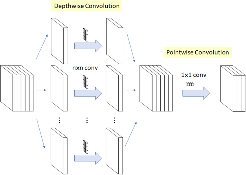
This efficient operation breaks a standard convolution into two distinct, much cheaper steps:

1. Depthwise Convolution: Performs spatial filtering for each input channel independently.
2. Pointwise Convolution: Combines the outputs from the depthwise step to create new features.

To get a clear visual intuition for this process, the following animation is invaluable.

Let's break down these two steps further.

Step 1: Depthwise Convolution

Imagine you have an input with 32 channels. A depthwise convolution will apply 32 separate 3x3x1 filters. The first filter slides over the first channel, the second filter over the second channel, and so on.

• Input: H x W x C_in
• Filters: F x F x 1 for each of the C_in channels. Total filters: C_in.
• Output: H' x W' x C_in

The key is that each filter is only "deep" by 1 channel. This stage only filters data spatially. It doesn't change the number of channels.

Step 2: Pointwise Convolution

The output of the depthwise step now needs its channels combined to form meaningful new features. This is done with a standard 1x1 convolution, which we've already seen in the Inception lesson. Since it operates on a single pixel location across all channels, it's often called a "pointwise" convolution in this context.

• Input: H' x W' x C_in (from the depthwise step)
• Filters: 1 x 1 x C_in for each of the C_out desired output channels. Total filters: C_out.
• Output: H' x W' x C_out

This step is purely about creating linear combinations of the channels. It has no spatial receptive field beyond a single "point".

3. Analyzing the Efficiency Gains

By splitting the operation, we achieve a massive reduction in computation and parameters. Let's quantify this. For a 3x3 convolution on an input feature map of size H x W x C_in producing an output of H x W x C_out:

• Standard Convolution Cost: 3 * 3 * C_in * C_out * H * W multiplications.
• Depthwise Separable Cost:
  1. Depthwise: 3 * 3 * C_in * H * W
  2. Pointwise: 1 * 1 * C_in * C_out * H * W
  3. Total: (3 * 3 * C_in + C_in * C_out) * H * W

The ratio of the cost is:

For any reasonable number of output channels (C_out), this ratio is significantly less than 1. For large C_out, the savings approach 9x for a 3x3 kernel!

The following article gives a very clear quantitative breakdown.

4. Designing MobileNet-Style Architectures

The MobileNet architecture family, developed by Google, is the primary showcase for depthwise separable convolutions. The first version, MobileNetV1, is essentially a deep stack of these efficient convolution blocks.

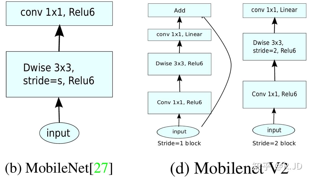
Let's implement this core block and then see how it's used to build the full network. Your experience with Python and building modular software will be helpful here.

Implementing the DepthwiseSeparableConv block

In PyTorch, a depthwise convolution is achieved by setting the groups parameter in nn.Conv2d to be equal to the number of input channels (groups=in_channels). This tells the layer to not mix information across channel groups, and since each channel is its own group, it results in a depthwise operation.

The following resource provides a complete, commented implementation of MobileNetV1 in PyTorch.

To see the underlying logic in a more fundamental way, outside of a deep learning framework, the following Python/NumPy code is illuminating.

MobileNetV1 demonstrates that by replacing nearly all standard convolutions with these efficient blocks, you can build a network that achieves competitive accuracy on tasks like ImageNet classification with a fraction of the computational budget.

Conclusion

You have now mastered the concept of depthwise separable convolutions, one of the most important architectural innovations for creating efficient deep learning models. We've moved beyond just making networks deeper or wider, and into the realm of making them smarter and more lightweight.

Key Takeaways:

• Separation of Concerns: Depthwise separable convolution splits a standard convolution into two stages: a depthwise stage for spatial filtering and a pointwise (1x1) stage for channel combination.
• Dramatic Efficiency Gains: This factorization reduces the number of parameters and computations by a factor of 8-9x compared to a standard 3x3 convolution, with only a minor trade-off in accuracy.
• MobileNet Architecture: This family of models is built almost entirely from depthwise separable convolution blocks, making them ideal for deployment on mobile phones and other edge devices.
• Implementation in PyTorch: A depthwise convolution can be implemented using nn.Conv2d by setting the groups parameter equal to the number of input channels.

Preview of the next lesson:
While MobileNet focuses on computational efficiency, other architectural patterns have emerged to improve feature representation itself. In our next lesson, we will apply dilated convolutions and squeeze-and-excitation networks for advanced feature extraction. Dilated convolutions allow us to expand the receptive field without increasing cost, while Squeeze-and-Excitation networks help the model focus on the most important feature channels.