Classic CNN Architectures: LeNet, VGG, and ResNet

Hello! Welcome back to our journey through the world of Convolutional Neural Networks.

Introduction

In our last lesson, you successfully built and trained your first CNN from scratch in PyTorch. You mastered the end-to-end workflow, from loading data to defining the model, writing the training loop, and evaluating performance. This provided you with a solid, practical foundation.

Today, we move from a generic "foundational" CNN to studying the giants whose shoulders modern computer vision stands upon. The goal for this lesson is to analyze and implement classic CNN architectures: LeNet, VGG, and ResNet. These aren't just historical footnotes; their design principles and architectural innovations are still fundamental to deep learning today. We will explore:

• LeNet: The pioneering architecture that proved the viability of CNNs.
• VGG: The model that demonstrated the power of sheer depth through a simple, elegant design.
• ResNet: The revolutionary architecture that introduced "skip connections" to break the depth barrier and enable networks hundreds of layers deep.

By the end of this lesson, you will understand the motivation, structure, and key contributions of each of these landmark models.

1. The Pioneer: LeNet-5

Our story begins in the 1990s with Yann LeCun's LeNet-5, an architecture designed for handwritten digit recognition on the MNIST dataset. It was one of the first commercially successful applications of neural networks and laid the conceptual groundwork for everything that followed.

The core ideas introduced in LeNet were foundational to all modern CNNs.

LeNet-5 combined these ideas into a straightforward sequence of layers. The architecture is simple enough to trace by hand.

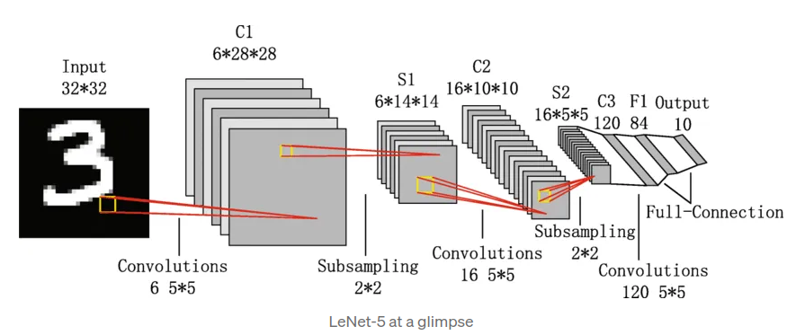
The architecture is as follows:

1. Input: 32x32 grayscale image.
2. C1 (Conv): 6 filters of size 5x5. Output: 6 feature maps of 28x28.
3. S2 (Subsampling/Avg Pooling): 2x2 pooling. Output: 6 feature maps of 14x14.
4. C3 (Conv): 16 filters of size 5x5. Output: 16 feature maps of 10x10.
5. S4 (Subsampling/Avg Pooling): 2x2 pooling. Output: 16 feature maps of 5x5.
6. C5 (Conv/Fully Connected): 120 filters of size 5x5. Output: 120 features.
7. F6 (Fully Connected): 84 units.
8. Output: 10 units (for 10 digits).

LeNet's success validated the CNN approach, but for over a decade, its potential was limited by the available data and computational power.

For a practical look at the implementation, the following resource provides a clean PyTorch version.

2. The Power of Depth: VGGNet

Fast forward to the 2010s. The ImageNet Large Scale Visual Recognition Challenge (ILSVRC) spurred a renaissance in computer vision. In 2012, AlexNet (a deeper, larger version of LeNet) won by a huge margin, kickstarting the deep learning revolution.

Two years later, VGGNet from the Visual Geometry Group at Oxford asked a simple question: How important is network depth? Their answer was a family of models (most famously VGG-16 and VGG-19) that pushed depth to 16-19 layers.

The key design philosophy of VGG was simplicity and uniformity.

• It exclusively uses very small 3x3 convolutional filters.
• Max pooling layers of size 2x2 with a stride of 2 are used to halve the spatial dimensions.
• The number of channels doubles after each pooling step.

Why use stacks of small 3x3 filters instead of one larger one (e.g., 5x5 or 7x7)?

1. Increased Non-linearity: A stack of two 3x3 conv layers has two ReLU activations, while a single 5x5 layer has only one. More non-linearity allows the model to learn more complex functions.
2. Fewer Parameters: A 5x5 conv layer has 5*5 = 25 parameters (per channel). A stack of two 3x3 layers has 2 * (3*3) = 18 parameters. This makes the network more efficient.
3. Equivalent Receptive Field: A stack of two 3x3 conv layers has an effective receptive field of 5x5, and a stack of three has a 7x7 field. They capture the same spatial context with the benefits above.

Test your understanding!

A single convolutional layer with a 7x7 kernel has a 7x7 receptive field.

Question: How many stacked 3x3 convolutional layers (with stride 1) would you need to achieve an equivalent receptive field? What are the advantages of using the stacked approach over the single 7x7 layer?

Show answer

You would need three stacked 3x3 convolutional layers.

• Layer 1: 3x3 receptive field.
• Layer 2: Sees the 3x3 output of the first layer. A 3x3 kernel on this gives it a 5x5 receptive field relative to the input.
• Layer 3: Sees the 5x5 field of the second layer. A 3x3 kernel on this gives it a 7x7 receptive field relative to the input.

The advantages are:

1. Fewer parameters: 3 * (3*3*C*C) = 27*C^2 vs 7*7*C*C = 49*C^2 (ignoring biases, where C is channels).
2. More non-linearities: Three ReLU activations instead of one, increasing the model's expressive power.

To see how VGG is implemented, you can refer to the same repository as before.

3. Breaking the Depth Barrier: ResNet

VGG showed that depth was beneficial. But researchers soon hit a wall: simply stacking more layers on top of a "plain" network led to a degradation problem. Counter-intuitively, a 56-layer plain network performed worse on both training and test sets than a 20-layer one. This wasn't overfitting; the deeper network was simply harder to train.

The breakthrough came from Microsoft Research in 2015 with ResNet (Residual Network). The solution was an elegant architectural tweak: the residual block.

The core idea is to learn a residual function instead of the direct mapping.

• A plain layer tries to learn a mapping H(x).
• A residual block learns F(x) = H(x) - x. The output is then computed as y = F(x) + x.

The x connection that bypasses the layers is called a skip connection or shortcut.

Why does this work? Imagine the identity mapping is optimal (i.e., H(x) = x). For a plain network, the layers must learn to approximate the identity function, which is difficult. For a residual block, the layers can simply learn to output zero (F(x) = 0), which is trivial. This makes it easy for the network to "skip" layers that are not useful, allowing for the training of much deeper models without degradation.

This skip connection also provides a direct path for gradients to flow during backpropagation, mitigating the vanishing gradient problem that plagues very deep networks.

Implementing ResNet is more involved than LeNet or VGG. It requires careful handling of the skip connections, especially when the input and output dimensions don't match (requiring a projection, often a 1x1 convolution, on the shortcut path).

The following video provides a superb from-scratch implementation in PyTorch. Given your background, walking through this code will be highly instructive.

Conclusion

Today you've traced the evolution of CNNs through three of its most important milestones. You saw how the field progressed from a simple proof-of-concept to grappling with, and ultimately solving, the challenge of training truly deep networks.

Key Takeaways:

• LeNet established the fundamental pattern of Conv -> Pool -> FC and proved the effectiveness of local receptive fields and shared weights.
• VGG demonstrated that depth is a critical component of performance, establishing a simple, uniform design principle of stacking 3x3 convolutions.
• ResNet introduced residual connections (skip connections) to solve the degradation problem, enabling the training of networks with hundreds or even thousands of layers and fundamentally changing how we design deep learning models.

Preview of the next lesson:
While VGG and ResNet focused on making networks deeper, another influential architecture from the same era, GoogLeNet, explored making them wider. In the next lesson, we will implement advanced architectural patterns like Inception modules, the core component of GoogLeNet. You'll learn a different design philosophy focused on parallel convolutions and computational efficiency.