Building a Basic CNN for Image Classification

Hello! Let's dive back into our study of Convolutional Neural Networks.

Introduction

In our last two lessons, you mastered the fundamental mechanics of CNNs. First, you implemented 2D convolution and pooling from scratch, giving you a firm grasp of how kernels, strides, and padding manipulate image data. Then, you analyzed the concept of the receptive field, understanding why we stack these layers: to build a hierarchical understanding of images, from simple edges to complex objects.

Today, we will synthesize all that knowledge. The goal of this lesson is to build a foundational CNN for an image classification task. We'll move from theory and individual components to constructing a complete, working system using the popular PyTorch framework. You will learn the entire workflow of a supervised deep learning project:

1. Loading and preparing a dataset.
2. Defining a network architecture.
3. Setting up the training process (loss function and optimizer).
4. Writing the training loop.
5. Evaluating the model's performance.

By the end of this lesson, you will have built and trained your first image classifier, a cornerstone skill in AI and computer vision.

Let's begin with a look at the overall architecture we're aiming to build.

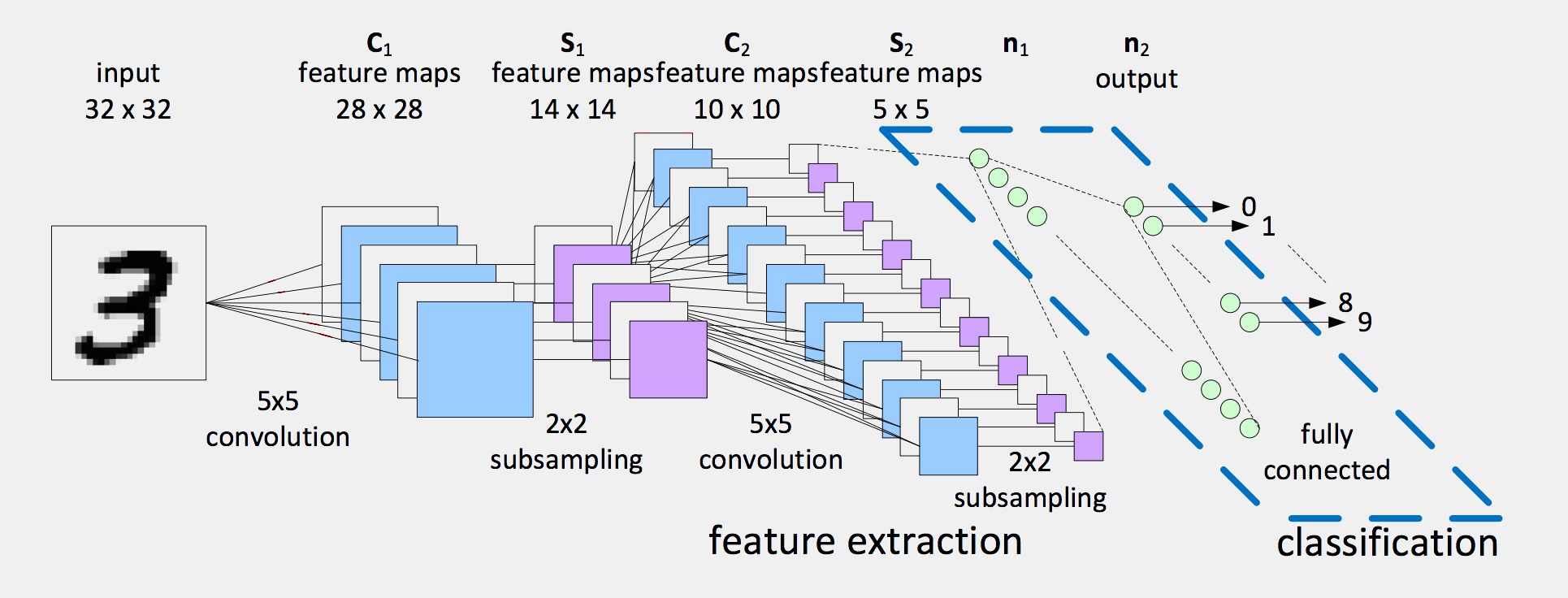
1. The Full Pipeline: From Data to Predictions

Training an image classifier involves a standardized set of steps. We'll walk through each one, using PyTorch to handle the implementation details. This will allow you to focus on the high-level structure and logic, leveraging your Python expertise.

We'll use the CIFAR-10 dataset, a classic benchmark in computer vision. It contains 60,000 32x32 color images across 10 classes, such as 'airplane', 'dog', 'car', etc.

The official PyTorch documentation provides an excellent tutorial that mirrors the steps we will take. We will use it as our primary textual reference.

2. Step 1: Loading and Normalizing Data

Before we can train a model, we need to prepare our data. This involves two main tasks:

• Loading the data: Getting the images and their corresponding labels from disk.
• Preprocessing the data: Applying transformations to make the data suitable for the network. The two essential transformations are:
  1. To Tensor: Converting the images, which are typically loaded as PIL (Python Imaging Library) objects, into PyTorch's native Tensor format.
  2. Normalization: Scaling the pixel values. Image pixels usually range from [0, 255]. They are first scaled to [0, 1], then normalized to [-1, 1] with a mean of 0.5 and a standard deviation of 0.5. This helps the model train faster and more stably.

PyTorch's torchvision library makes this process incredibly convenient. We use torchvision.datasets to download and load CIFAR-10, and torch.utils.data.DataLoader to serve up the data in shuffled batches.

Let's watch a practical demonstration of this process.

As you saw, with just a few lines of code, we have a pipeline that automatically downloads, transforms, and serves batches of data for our training loop.

3. Step 2: Defining the CNN Architecture

Now, we define the structure of our neural network. In PyTorch, we do this by creating a class that inherits from torch.nn.Module. This class has two essential methods:

• __init__(): The constructor, where we define all the layers our network will use (e.g., Conv2d, Linear).
• forward(self, x): This method defines the forward pass. It dictates how the input tensor x flows through the layers defined in __init__().

Our network will consist of two main blocks:

1. Feature Extractor: A sequence of Conv2d, ReLU, and MaxPool2d layers. This is where the network learns to identify visual patterns, from simple edges to more complex textures. The feature maps from these layers are what you saw visualized in the image below.
2. Classifier: A sequence of Linear (fully connected) layers that take the flattened features from the extractor and make a final prediction.

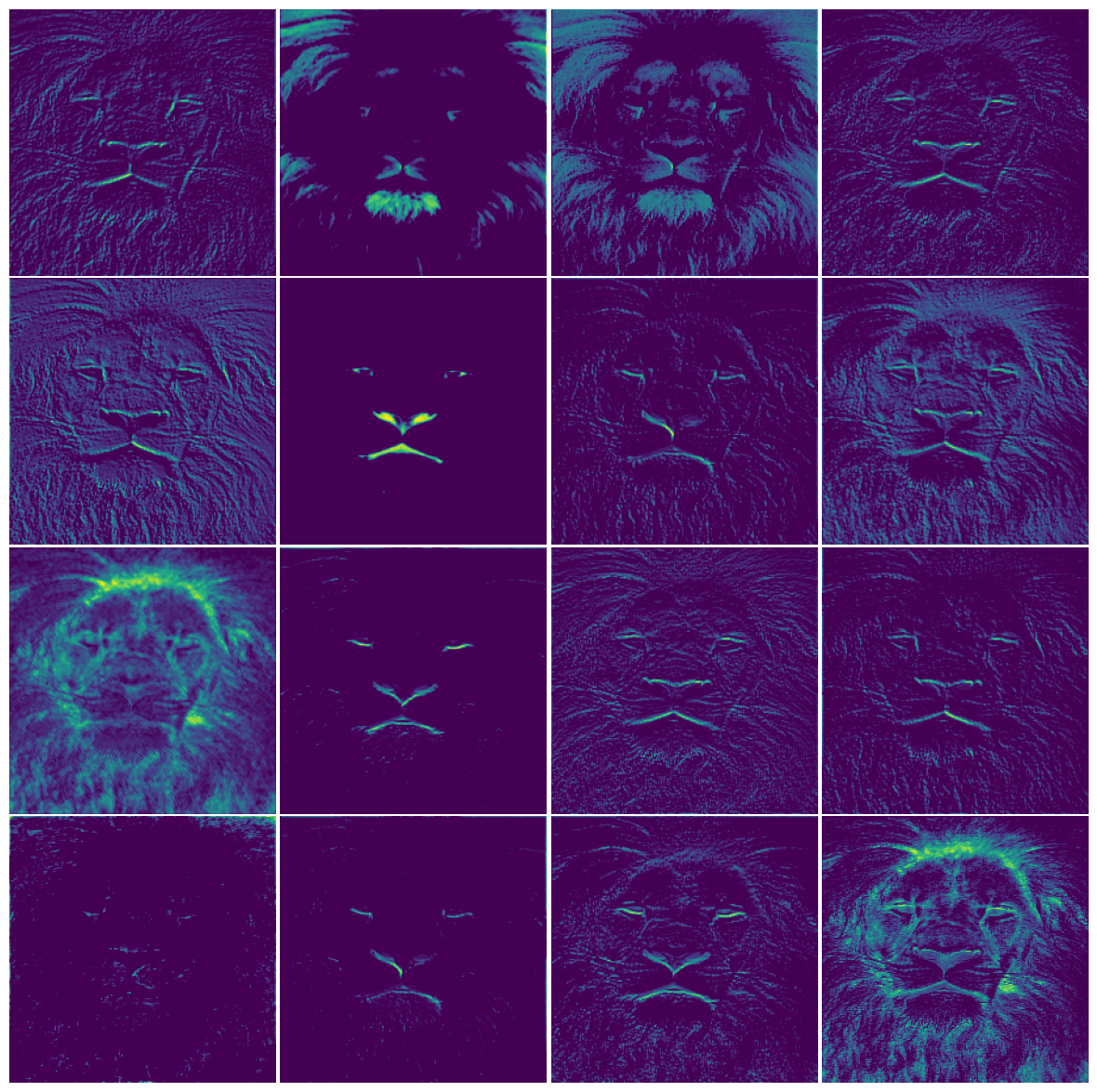
A critical step is flattening the output of the convolutional block. The Conv2d layers produce 3D tensors (channels x height x width), but the Linear layers expect a 1D vector. The flatten operation reshapes the tensor, preparing it for the classifier.

The following segments of the video show how to implement this in PyTorch.

You can also find the complete code for a similar network in the official PyTorch tutorial.

Test your understanding!

In the Net class from the PyTorch tutorial, the first linear layer is self.fc1 = nn.Linear(16 * 5 * 5, 120). The 16 * 5 * 5 is derived from the output shape of the second pooling layer.

Let's trace the tensor shape. The input image is 3x32x32.

• conv1 (k=5) + pool1 (k=2, s=2):
  • After conv1, size = 32 - 5 + 1 = 28. Shape is now 6x28x28.
  • After pool1, size = 28 / 2 = 14. Shape is now 6x14x14.
• conv2 (k=5) + pool2 (k=2, s=2):
  • After conv2, size = 14 - 5 + 1 = 10. Shape is now 16x10x10.
  • After pool2, size = 10 / 2 = 5. Shape is now 16x5x5.
• This 16x5x5 tensor is flattened into a vector of size 16 * 5 * 5 = 400.

Question: How would you calculate the input size for self.fc1 if you modified self.conv2 to have 32 output channels and a kernel size of 3x3 (with stride 1 and no padding)? All other layers remain the same.

Show answer

Let's trace the shape again with the new conv2.

• Input shape entering conv2 is 6x14x14.
• conv2 is now nn.Conv2d(6, 32, 3).
  • The output spatial dimension will be 14 - 3 + 1 = 12.
  • The output shape from conv2 is now 32x12x12.
• pool2 (k=2, s=2) is applied to this 32x12x12 tensor.
  • The output spatial dimension will be 12 / 2 = 6.
  • The final shape before flattening is 32x6x6.
• The flattened vector size would be 32 * 6 * 6 = 1152.

So, the new linear layer would be self.fc1 = nn.Linear(1152, 120). This exercise is crucial for correctly connecting your convolutional layers to your dense layers.

4. Step 3 & 4: Loss, Optimizer, and the Training Loop

With the data and model defined, we need to set up the training machinery.

• Loss Function: Since this is a multi-class classification problem, we use nn.CrossEntropyLoss. This loss function is ideal because it combines LogSoftmax and Negative Log-Likelihood Loss, making it numerically stable and convenient. It expects the raw, unnormalized outputs (logits) from the model.
• Optimizer: This is the algorithm that updates the model's weights based on the gradients calculated during backpropagation. We'll start with a classic: optim.SGD (Stochastic Gradient Descent) with momentum.

The training loop is the heart of the process. It iterates over the training data for a set number of epochs (one epoch = one full pass through the dataset). For each batch in the dataset, it performs these five essential steps:

1. Zero Gradients: optimizer.zero_grad(). Clear the gradients from the previous batch.
2. Forward Pass: outputs = net(inputs). Pass the input data through the model to get predictions.
3. Compute Loss: loss = criterion(outputs, labels). Compare the model's predictions to the true labels.
4. Backward Pass: loss.backward(). This is where PyTorch's autograd engine automatically computes the gradients of the loss with respect to all model parameters.
5. Update Weights: optimizer.step(). The optimizer uses the computed gradients to update the model's weights.

Let's see this implemented.

5. Step 5: Evaluating the Model

After training, we must test the model on data it has never seen: the test set. This gives us an unbiased measure of its generalization performance. The evaluation loop is similar to the training loop but simpler:

1. Set the model to evaluation mode: net.eval(). This turns off layers like Dropout or BatchNorm that behave differently during training.
2. Disable gradient calculation with with torch.no_grad(): for speed and memory efficiency.
3. Loop through the test data, perform a forward pass, and get predictions.
4. Instead of calculating loss, we compare the predicted class with the ground truth label to calculate accuracy.

The video below demonstrates how to evaluate the model, save its trained weights, and even use it to classify new images from the web.

An Alternative: The TensorFlow/Keras Approach

As an engineer, it's valuable to know that different frameworks offer different levels of abstraction. The PyTorch approach you just learned gives you explicit control over the training loop. TensorFlow's high-level API, Keras, abstracts this away into a simple .fit() method.

The video below demonstrates the Keras approach. You don't need to study it in detail, but observing the difference is insightful.

Conclusion

Congratulations! You have now walked through the entire process of building, training, and evaluating a foundational Convolutional Neural Network for image classification. You've translated the theoretical concepts of convolution, pooling, and receptive fields into a practical, working system.

Key Takeaways:

• The standard workflow for a supervised learning task is: Data Prep -> Model Definition -> Loss/Optimizer Setup -> Training Loop -> Evaluation.
• In PyTorch, a CNN is defined as a class inheriting from nn.Module, with layers in __init__ and data flow in forward.
• The training loop consists of a repeating cycle: zero_grad(), forward(), loss.backward(), optimizer.step().
• Data preprocessing, especially normalization and tensor conversion, is a critical first step.
• The transition from convolutional layers to dense layers requires a flatten operation, and calculating the correct tensor dimensions is crucial.

Preview of the next lesson:
The simple CNN we built is a great starting point, but modern computer vision relies on much deeper and more sophisticated architectures. In our next lesson, we will analyze and implement classic CNN architectures: LeNet, VGG, and the revolutionary ResNet. You will see how these models solved key challenges like training very deep networks and learn architectural patterns that are still relevant today.