Understanding Receptive Fields in CNNs

Hello! Welcome back to our module on Convolutional Neural Networks.

Introduction

In our last lesson, you did an excellent job implementing the core 2D convolution and pooling operations from scratch. You now have a solid, low-level understanding of how kernels, padding, and stride work to transform an input image or feature map.

Today, we'll build directly on that knowledge to answer a crucial question: What is the benefit of stacking these layers? The answer lies in the concept of the receptive field. By stacking layers, a CNN builds a hierarchy of features—from simple edges and textures in early layers to complex object parts in later layers. The receptive field is the mechanism that allows a neuron in a deep layer to "see" and integrate information from a large region of the original input image.

Your learning outcome for this lesson is to analyze the concept of receptive fields in CNNs. By the end, you will be able to:

Define and visualize how a neuron's receptive field expands through the layers of a network.
Calculate the size of the theoretical receptive field based on a network's architecture.
Explain the difference between the theoretical and the more practical effective receptive field.
Understand why the receptive field is a critical parameter in CNN design for tasks like object recognition.

1. The Cascading View of a CNN

A neuron in a convolutional layer gets its input from a small patch of the previous layer, determined by the kernel size. But what about the neurons in that previous layer? They, in turn, received their input from patches of the layer before them. This creates a cascading effect. A single neuron deep in the network can synthesize information from a progressively larger region of the original input. This "field of view" into the input layer is its receptive field.

Let's start with a short video that provides a clean, high-level intuition for this concept.

What is the Receptive Field in Convolutional Neural Networks?

The video 'What is the Receptive Field in Convolutional Neural Networks?' by Johannes Frey offers a great qualitative explanation.

Please watch from 02:18 to 03:38. Focus on the idea that a convolution in a deeper layer operates on a 'condensed version' of the original image, which effectively widens its view.

Now, let's make this more concrete with an animated visualization. The following video beautifully illustrates the receptive field growing through a simple 3-layer CNN.

CNN Receptive Field | Deep Learning Animated

The video 'CNN Receptive Field | Deep Learning Animated' from Deepia provides an excellent step-by-step visualization of the growing receptive field.

Please watch from 01:19 to 03:04. Observe how a 3x3 window in the second layer corresponds to a 5x5 region in the input, and a 3x3 window in the third layer corresponds to a 7x7 region.

As you can see, each successive layer sees a wider context. This is how CNNs build a hierarchical understanding of an image:

Layer 1: Detects simple patterns (edges, corners, colors) within small 3x3 or 5x5 receptive fields.
Layer 2: Combines these simple patterns into more complex textures or parts of objects (e.g., combining an edge and a curve to form an eye) within a larger receptive field.
Deeper Layers: Combine these parts into full objects (e.g., eyes, nose, and mouth into a face) within a very large receptive field that might cover a significant portion of the image.

2. Calculating the Theoretical Receptive Field

This growth isn't random; it can be calculated precisely. The size of the receptive field is a function of the kernel sizes and strides of all preceding layers. Let's get into the mathematics.

The Recurrence Formula

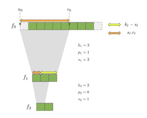
Consider a network with $L$ layers. Let $r_{l}$ be the receptive field size with respect to layer $l$ . We want to find $r_{0}$ , the receptive field size with respect to the input image.

We can define the receptive field size recursively. The receptive field of a neuron in layer $l$ with respect to the previous layer, $l - 1$ , is simply its kernel size, $k_{l}$ . To find the receptive field with respect to layer $l - 2$ , we have to consider how far apart the neurons in layer $l - 1$ were, which is determined by the stride $s_{l - 1}$ .

A general recurrence relation for the receptive field size $r$ at layer $l - 1$ in terms of layer $l$ is:

$r_{l - 1} = s_{l} \cdot (r_{l} - 1) + k_{l}$

This formula can be a bit unintuitive. A more straightforward way to think about it is to start from the output and work backward. The excellent article "Computing Receptive Fields of Convolutional Neural Networks" from Distill.pub provides a very clear derivation.

Computing Receptive Fields of Convolutional Neural Networks

This article from Distill.pub is a definitive guide to the mathematics of receptive fields. We'll focus on the section that derives the formula for a simple, single-path network.

Please read the section titled 'Computing receptive field size'. Focus on understanding the intuition behind the final closed-form expression (Equation 2): r_0 = \sum_{l=1}^{L} \left((k_l-1)\prod_{i=1}^{l-1} s_i\right) + 1 Don't worry about memorizing it, but try to grasp what each part represents: (k_l-1) is the size added by a layer, and the product of strides Π s_i scales this addition based on its position in the network.

Let's break down that closed-form equation:

$r_{0}$ : The final receptive field size on the input image.
$l$ : The index of the current layer we are considering (from 1 to $L$ ).
$k_{l}$ : The kernel size of layer $l$ .
$s_{i}$ : The stride of a preceding layer $i$ .

The formula essentially says: start with a receptive field of size 1. Then, for each layer $l$ , add k_l - 1 to the receptive field. However, this addition must be "magnified" by the product of the strides of all layers that came before it.

The Impact of Stride and Pooling

The most important takeaway from the formula is the role of the stride, $s$ . Since strides are multiplied, a stride greater than 1 (e.g., $s = 2$ ) in an early layer will exponentially increase the receptive field of all subsequent layers.

This is why pooling layers are so powerful for expanding the receptive field. A 2x2 pooling operation with a stride of 2 is, for the purpose of receptive field calculation, equivalent to a convolutional layer with a kernel size $k = 2$ and a stride $s = 2$ . It effectively doubles the receptive field growth rate.

Let's see this demonstrated.

CNN Receptive Field | Deep Learning Animated

Let's return to the 'CNN Receptive Field' video, which has a great segment explaining the calculation and the impact of pooling.

Watch from 03:04 to 07:23. Pay close attention to how the formula is applied and, crucially, how adding pooling layers causes the receptive field to grow exponentially.

Test your understanding!

Let's calculate the receptive field of a neuron in the final feature map of this simple network:

Input Image: 28x28
Layer 1 (Conv): Kernel k=5, Stride s=1
Layer 2 (Pool): Kernel k=2, Stride s=2
Layer 3 (Conv): Kernel k=3, Stride s=1

What is the receptive field size $r_{0}$ ?

Show answer

Let's use the closed-form formula: $r_{0} = \sum_{l = 1}^{L} ((k_{l} - 1) \prod_{i = 1}^{l - 1} s_{i}) + 1$

For Layer 1 (l=1):
- Contribution = $(k_{1} - 1) \times 1$ (product of strides before layer 1 is empty, so it's 1)
- Contribution = $(5 - 1) \times 1 = 4$
For Layer 2 (l=2):
- Contribution = $(k_{2} - 1) \times s_{1}$
- Contribution = $(2 - 1) \times 1 = 1$
For Layer 3 (l=3):
- Contribution = $(k_{3} - 1) \times (s_{1} \times s_{2})$
- Contribution = $(3 - 1) \times (1 \times 2) = 2 \times 2 = 4$
Total size $r_{0}$ :
- $r_0 = (\text{contribution_1} + \text{contribution_2} + \text{contribution_3}) + 1$
- $r_{0} = (4 + 1 + 4) + 1 = 10$

The receptive field of a neuron in the output of Layer 3 is 10x10 pixels on the original input image.

3. The Effective Receptive Field

So far, we've discussed the theoretical receptive field, which assumes every pixel within that computed boundary has an equal influence. In reality, this is not the case.

The pixels at the center of a receptive field have many more "paths" through the network to influence the final output neuron compared to pixels at the edge. This leads to the concept of the effective receptive field (ERF): the region of the input that actually has a significant, non-negligible impact on the output.

The ERF has two surprising properties:

It has a Gaussian shape, meaning the influence of pixels drops off rapidly as you move from the center to the edge of the theoretical receptive field.
In deep networks, the size of the ERF grows much more slowly ( $O (L)$ ) than the theoretical RF ( $O (L)$ ). This means the ERF is often a small fraction of the theoretical RF.

Let's watch a final clip that explains and visualizes the ERF.

CNN Receptive Field | Deep Learning Animated

The 'CNN Receptive Field' video also provides a clear explanation of the effective receptive field and how it differs from the theoretical one.

Watch from 07:23 to the end (10:16). Note how the ERF is visualized using backpropagation and how its shape changes during training.

For a deeper dive into this fascinating topic, the original research paper, "Understanding the Effective Receptive Field in Deep Convolutional Neural Networks," established these properties. Its key insight comes from modeling the influence as a partial derivative, $\frac{\partial output}{\partial input}$ , and showing its distribution.

Understanding the Effective Receptive Field in Deep Convolutional Neural Networks

Let's briefly look at the original paper that introduced the ERF. We'll focus on the core ideas, not the full mathematical proofs.

Skim through the following sections to grasp the main points: Section 1 (Introduction): Understand the motivation for studying the receptive field more deeply. Section 2 (Properties of Effective Receptive Fields): Note that the measure of impact is defined as the partial derivative \frac{\partial y_{0,0}}{\partial x^0_{i,j}}. Section 2.3 (Non-uniform kernels): Read the paragraph connecting the analysis to the Central Limit Theorem and the conclusion that the ERF size grows as O(\sqrt{n}) while the theoretical RF grows linearly. Section 3.2 (How the ERF evolves during training): Look at Figure 3. It shows that while the ERF starts small, it actually grows significantly during the training process as the network learns what features are important.

This is a critical insight: while architectural choices determine the potential receptive field, the training process itself shapes the effective receptive field, expanding it to focus on relevant information.

4. Application in Network Design

Understanding receptive fields is not just a theoretical exercise; it's fundamental to designing effective CNNs.

Task-Appropriate Scale: The receptive field of the final convolutional layer must be large enough to encompass the objects of interest. For classifying large objects in ImageNet, you need a very large receptive field. For finding small texture defects in a material, a smaller RF might be sufficient.
Architectural Trends: The push towards deeper networks (like VGG, ResNet) and the widespread use of pooling and strided convolutions are direct consequences of the need for large receptive fields. The Distill.pub article includes a table showing the massive receptive fields of modern architectures. For example, ResNet-152 has a theoretical receptive field of 1507x1507 pixels! This allows it to use context from the entire image to make a decision about a single feature.

Receptive Field Expansion in a 1D CNN — This diagram provides a static, 1D visualization of receptive field expansion. A neuron in the final layer (`f2`) is influenced by a region in `f1`, which in turn is influenced by a wider region in the input `f0`. The final receptive field is the total span on `f0` required to compute that single output value.

Conclusion

You've now analyzed one of the most important concepts for understanding how CNNs "see." This bridges the gap between individual layer operations and the holistic behavior of a deep network.

Key Takeaways:

The receptive field is the region of the input image that influences a specific neuron's output.
Stacking convolutional and pooling layers causes the receptive field to grow, allowing the network to learn a hierarchy of features from simple to complex.
The theoretical receptive field can be precisely calculated based on the network's kernel sizes and strides. Stride has a multiplicative effect on growth.
The effective receptive field is the region that actually influences the output. It is typically Gaussian-shaped and smaller than its theoretical counterpart, but it grows and adapts during training.
Designing a network with an appropriate receptive field size is crucial for a model's success on a given computer vision task.

Preview of the next lesson:
We have all the conceptual pieces in place. You know how to implement the building blocks (conv, pool) and you understand the key design principle that governs how they are stacked (receptive field). In the next lesson, we will put it all together to build a foundational CNN for an image classification task. We'll move from implementing single operations to defining a full nn.Module in a framework like PyTorch, and train it on a real dataset.