Building Blocks of CNNs: Conv & Pooling from Scratch

Hello! Welcome to the first lesson in our new module, Convolutional Neural Networks for Computer Vision.

Introduction

In the previous module, we built a solid foundation in deep neural networks, culminating in strategies like early stopping and learning rate scheduling to train them effectively. We worked primarily with Multi-Layer Perceptrons (MLPs), which are powerful but have a significant limitation: they expect flattened vector inputs. This isn't ideal for data like images, where the spatial arrangement of pixels contains crucial information. Flattening an image throws away this spatial structure.

Today, we dive into the architecture specifically designed to understand spatial data: the Convolutional Neural Network (CNN). We'll start at the very heart of CNNs by exploring their fundamental building blocks.

Your learning outcome for this lesson is to implement 2D convolution and pooling operations from scratch. By the end, you'll understand:

• The core concept of a 2D convolution as a feature-detecting filter.
• The mechanics of the operation, including kernels, padding, and stride.
• The purpose and function of pooling for downsampling.
• How to implement the forward pass for both operations using Python and NumPy.

This hands-on, "from scratch" approach will give you a deep and lasting understanding of how CNNs process visual information, setting the stage for building and analyzing complex vision models.

1. The Intuition Behind Convolution

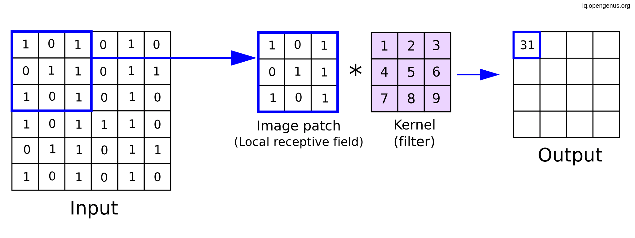
At its core, a convolution is an operation that uses a small matrix, called a kernel or filter, to slide over an image and extract specific features. Think of a kernel as a magnifying glass that is specialized to find one particular thing, like a vertical edge, a horizontal line, or a specific color pattern.

By sliding this kernel over every part of the image, we create a new "filtered" image, or feature map, that highlights where the feature was detected.

Let's watch a short video that provides a high-level, intuitive overview of convolutions and how they serve as feature detectors.

As the video explains, a CNN doesn't use pre-defined filters. Instead, it learns the optimal values for the kernels during training—the same way an MLP learns its weights. The network itself discovers which features are most useful for a given task.

2. The Mechanics of 2D Convolution

To implement convolution, we need to understand its mechanical details: how the kernel moves, how we handle image boundaries, and how it works with color images.

2.1 Convolution vs. Cross-Correlation

A quick but important technical point. The operation we just described—sliding a kernel and computing a sum of element-wise products—is technically called cross-correlation. A true mathematical convolution involves flipping the kernel by 180 degrees before applying it.

In deep learning, frameworks like PyTorch and TensorFlow implement cross-correlation but call the layer "Convolution". Why? Because the network can learn a flipped version of the kernel just as easily. For the forward pass, it makes no practical difference to the model's expressive power. However, for a "from scratch" implementation and for understanding the math of backpropagation later, this distinction is critical.

Let's watch a short segment that clarifies this.

For the rest of this lesson, we will implement the cross-correlation operation, as this is standard practice for the forward pass of a CNN layer.

2.2 Padding and Stride

Two key hyperparameters control the behavior of the convolution and the size of the output feature map:

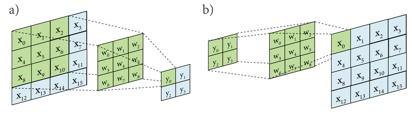
1. Padding: If we apply a kernel to an image, the output feature map will be smaller than the input. To prevent this shrinking (which can be problematic in deep networks) and to give more importance to the pixels at the edge of the image, we can add a border of zeros around the input. This is called zero-padding.
2. Stride: This is the step size the kernel takes as it slides across the image. A stride of 1 means the kernel moves one pixel at a time. A stride of 2 means it moves two pixels at a time, which will result in a smaller output map.

The dimensions of the output feature map can be calculated with these formulas:

$n_H^{out}=\lfloor \frac{n_H^{in}-f+2p}{s}\rfloor +1$
$n_W^{out}=\lfloor \frac{n_W^{in}-f+2p}{s}\rfloor +1$

where:

• $n_H^{in},n_W^{in}$ are the height and width of the input.
• $f$ is the size of the kernel (e.g., 3 for a 3x3 kernel).
• $p$ is the amount of padding.
• $s$ is the stride.

Test your understanding!

You have an input image of size 32x32. You apply a 5x5 kernel with a stride of 1 and padding of 2. What is the size of the output feature map?

Show answer

Using the formula:
$n_H^{out}=\lfloor \frac{32-5+2\times 2}{1}\rfloor +1=\lfloor \frac{31}{1}\rfloor +1=32$
$n_W^{out}=\lfloor \frac{32-5+2\times 2}{1}\rfloor +1=\lfloor \frac{31}{1}\rfloor +1=32$

The output size is 32x32. Notice that with p = (f-1)/2, we preserve the input dimensions. This is often called "same" padding.

2.3 Multi-Channel Convolution

Real-world images have multiple channels (e.g., Red, Green, and Blue for RGB). How does convolution work then?

• The input is a 3D volume: (height, width, channels).
• The kernel must also be a 3D volume with the same number of channels as the input: (kernel_size, kernel_size, input_channels).
• During the operation, the 2D slices of the kernel are applied to the corresponding 2D slices (channels) of the input. The results are then summed up (along with a single bias term) to produce a single value in the output.
• This means that even with a multi-channel input, a single kernel produces a 2D feature map.
• To get a multi-channel output, we simply use multiple kernels. If we use D different kernels, we will get D output channels.

This is a crucial concept, and the next video segment has an excellent animation that makes it crystal clear.

3. Implementing the Convolution Forward Pass

Now, let's translate this into code. We'll implement the forward pass of a convolution layer using NumPy. We'll follow a step-by-step guide that breaks the problem down into manageable functions.

The implementation in that guide uses a series of for loops. Given your background in software engineering, you might recognize this as a clear but potentially inefficient approach. In practice, deep learning libraries use highly optimized algorithms (like im2col) to convert the convolution into a single large matrix multiplication, which can be massively parallelized on a GPU. However, for understanding the mechanics, this looped implementation is perfect.

For an alternative perspective, the article "Building a Convolutional Neural Network(CNN) From Scratch" (resource ID LINK) encapsulates this logic within a Python class, which is a common way to structure layers in a neural network framework. Feel free to browse its convolution class for comparison.

4. The Pooling Operation

After a convolution operation, it's common to add a pooling layer. The main purpose of pooling is to downsample the feature maps, making them smaller. This has two key benefits:

1. It reduces the number of parameters and computations in the network, making it more efficient.
2. It makes the feature representations somewhat invariant to small translations in the input image. If the feature moves slightly, the pooled output might not change.

The most common types of pooling are:

• Max Pooling: Slides a window over the feature map and takes the maximum value from the window. This is effective at preserving the most prominent features.
• Average Pooling: Takes the average of all values in the window. This provides a smoother, more general downsampling.

Let's watch the second half of the Google for Developers video to see pooling in action.

Like convolution, pooling is defined by a window size and a stride. It typically does not involve padding.

Test your understanding!

Given the following 4x4 feature map, what is the output after applying a 2x2 max pooling with a stride of 2?

$$\left(\begin{array}{cccc}1& 3& 2& 4\\ 8& 5& 0& 6\\ 3& 1& 9& 2\\ 7& 4& 6& 5\end{array}\right)$$

Show answer

We process the matrix in 2x2 blocks:

• Top-left block: [[1, 3], [8, 5]]. Max is 8.
• Top-right block: [[2, 4], [0, 6]]. Max is 6.
• Bottom-left block: [[3, 1], [9, 2]]. Max is 9.
• Bottom-right block: [[7, 4], [6, 5]]. Max is 7.

The resulting 2x2 pooled feature map is:

$$\left(\begin{array}{cc}8& 6\\ 9& 7\end{array}\right)$$

5. Implementing the Pooling Forward Pass

The implementation of pooling is very similar to convolution, but simpler since there are no weights or biases to consider—just a sliding window and an aggregation function (max or mean).

Let's return to our step-by-step guide to see the implementation.

Conclusion

Excellent work! You have now implemented the two most fundamental operations in any Convolutional Neural Network from scratch. This low-level understanding is invaluable as we start assembling these blocks into powerful deep learning models for vision.

Key Takeaways:

• 2D Convolution is a feature detection operation that slides a learned kernel over an input feature map. It's technically cross-correlation in most deep learning libraries.
• The output size is controlled by the input size, kernel size, padding, and stride.
• Multi-channel convolutions use kernels with the same depth as the input to produce 2D feature maps. Multiple kernels create a multi-channel output.
• Pooling (Max or Average) is a downsampling operation that reduces the spatial dimensions of feature maps, providing efficiency and some translational invariance.
• Both operations can be implemented with nested loops that define a sliding window and apply a specific computation within that window.

Preview of the next lesson:
Now that we've seen how to build a single convolutional or pooling layer, what happens when we stack them? Stacking these layers allows a CNN to build a hierarchy of features, from simple edges to complex objects. A key concept for understanding this process is the receptive field. In our next lesson, we will analyze how the receptive field of a neuron grows as we go deeper into a CNN, enabling it to "see" and understand larger and more abstract patterns in the input image.