LLM-d Architecture & Extreme Scale Use Cases

Introduction

In the last few lessons, you've surveyed the leading production inference frameworks: vLLM, SGLang, and TensorRT-LLM. While they differ in their execution models—dynamic interpretation vs. ahead-of-time compilation—they all operate on a similar principle: a model is served by a tightly-coupled set of workers, typically running on one or more GPUs in a single machine or a tightly-networked cluster.

Today, we will explore a fundamentally different paradigm designed for extreme scale: disaggregated serving. This architectural pattern challenges the assumption that all parts of the inference process must run on the same hardware. We'll find that by splitting the process into its constituent parts, we can solve deep-seated performance issues that even sophisticated frameworks like vLLM struggle with under certain conditions.

Your goal for this lesson is to explain the disaggregated serving architecture of systems like LLM-d and identify their target use cases for extreme scale. You will learn why a seemingly more complex architecture can lead to massive gains in efficiency and performance, particularly for the demanding workloads that are becoming increasingly common.

The Core Problem: Throughput vs. Goodput

For a long time, raw throughput (tokens/second) was the primary metric for inference performance. However, in user-facing applications, latency is just as important. A system that generates many tokens per second is useless if users abandon their requests because the initial response takes too long or the words appear too slowly.

This brings us to two critical Service Level Objectives (SLOs):

• Time To First Token (TTFT): The latency from when a request is sent until the first output token is received.
• Time Per Output Token (TPOT) or Inter-Token Latency (ITL): The average latency between subsequent output tokens.

A better metric for serving performance, which accounts for these SLOs, is goodput: the number of requests per second that meet their TTFT and TPOT targets.

To understand this concept and why it's so important, let's watch the introduction to a talk on DistServe, one of the pioneering academic systems in this area.

The central question, then, is: why do modern serving systems, even with optimizations like continuous batching, struggle to maximize goodput? The answer lies in the conflicting nature of the two main phases of inference: prefill and decode.

The Interference of Prefill and Decode

As you know from building an LLM from scratch, inference isn't a single, uniform process. It's a two-stage act:

1. Prefill: The input prompt is processed in a single, large forward pass. All tokens in the prompt are processed in parallel to generate the KV cache and the very first output token. This phase is heavily compute-bound. Its latency is proportional to the square of the prompt length, and even a single long prompt can saturate the GPU's computational units.
2. Decode: Subsequent tokens are generated one at a time, autoregressively. Each step is a small forward pass that appends one new token's state to the existing KV cache. This phase is heavily memory-bandwidth-bound. It involves moving large amounts of data (the model weights and the entire KV cache) for a relatively small amount of computation.

When you run both phases on the same GPU, they interfere with each other. A long, compute-heavy prefill task will hog the GPU's compute resources, causing latency-sensitive decode steps for other requests in the same batch to stall. This dramatically increases TPOT and can cause you to miss your SLOs, thus reducing your goodput.

For a detailed technical explanation of this interference, let's turn to a lecture by one of the researchers behind this work.

This interference creates a second problem: suboptimal resource allocation. The optimal parallelism strategy for compute-bound prefill (e.g., more tensor parallelism to reduce latency) is often different from the optimal strategy for memory-bound decode (e.g., more data parallelism to increase throughput). In a co-located system, you're forced to choose a single configuration that is a compromise for both.

The Solution: Disaggregated Serving

The solution to this interference and resource allocation problem is conceptually simple but architecturally profound: disaggregate the prefill and decode stages onto separate, specialized pools of hardware.

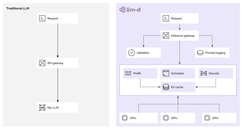
In a disaggregated architecture, the lifecycle of a request looks like this:

1. A request arrives at an intelligent gateway/scheduler.
2. The scheduler routes the prompt to a dedicated Prefill Worker.
3. The Prefill Worker executes the prefill step, generating the first output token and the full KV cache for the prompt.
4. The system orchestrates a high-speed transfer of this KV cache to a dedicated Decode Worker.
5. The Decode Worker takes over, performing the autoregressive decoding until the sequence is complete.

This design elegantly solves our two main problems:

• No Interference: The long, compute-intensive prefill tasks run in their own hardware pool and can no longer stall the latency-sensitive decode steps running in a different pool.
• Optimal Resource Allocation: You can provision each pool independently. The prefill pool can use GPUs and parallelism strategies optimized for compute, while the decode pool can be optimized for memory bandwidth and throughput.

To see a quantitative example of the benefit, let's return to the "GPU MODE" lecture. The speaker provides a clear, numerical walkthrough showing how disaggregation can double the goodput per GPU.

A Concrete System: llm-d

llm-d is an open-source project that brings this disaggregated architecture to production environments using Kubernetes. It integrates several industry-standard tools to create a robust, scalable serving stack.

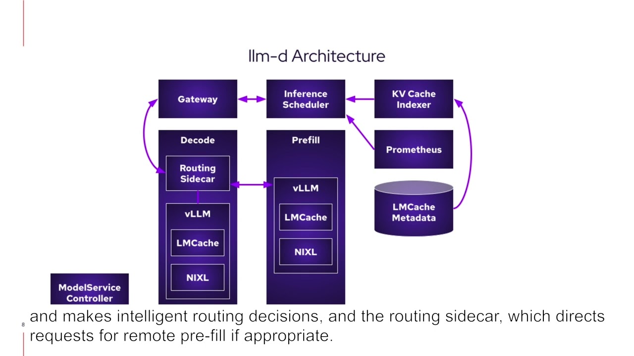
To understand how these pieces fit together, let's examine the official architecture documentation.

The scheduler is the heart of the llm-d system. It doesn't just blindly forward requests; it makes intelligent decisions based on the request's characteristics and the real-time state of the worker pools. For instance, a very short prompt might not benefit from disaggregation, as the overhead of transferring the KV cache would outweigh the benefits. In this case, the scheduler can route it to a single worker that handles both phases.

This blog post provides excellent, easy-to-follow examples of the scheduler in action.

Target Use Cases for Extreme Scale

The added architectural complexity of disaggregated serving is not a free lunch. It's a powerful tool designed for specific, challenging scenarios where traditional architectures fall short. The primary use cases include:

• Workloads with Long Prompts: This is the canonical use case. Applications involving Retrieval-Augmented Generation (RAG), long multi-turn conversations, or agentic systems with large system prompts all involve very long prefill stages. Disaggregation is crucial to prevent these long prefills from crippling the system's overall responsiveness (TPOT).
• Services with Strict and Diverse SLOs: A platform serving multiple applications may need to simultaneously support code completion (demanding ultra-low TTFT) and document summarization (demanding high TPOT). Disaggregation allows you to provision and scale the prefill and decode pools independently to meet these conflicting demands and maximize total system goodput.
• Extreme-Scale Models and Throughput: For very large models or services with massive request volumes, you can apply different parallelism strategies to each pool. For instance, you might use 4-way tensor parallelism in the prefill pool to slash TTFT, while using data parallelism across a larger number of replicas in the decode pool to maximize token generation throughput. This level of granular control is impossible in a co-located architecture.
• Heterogeneous Hardware Environments: Disaggregation opens the door to using different types of accelerators for each stage. You could use a GPU with superior compute performance (e.g., H100) for the compute-bound prefill stage, and a different GPU with higher memory bandwidth (e.g., a future HBM-focused chip) for the memory-bound decode stage, thus optimizing hardware cost and efficiency.

Conclusion

In this lesson, you've moved beyond monolithic serving architectures to understand the principles and practical implementation of disaggregated inference. This approach addresses the fundamental conflict between the compute-bound prefill phase and the memory-bound decode phase.

Key Takeaways:

• Goodput is the Goal: In real-world applications, performance is measured by goodput—throughput that meets latency SLOs (TTFT and TPOT)—not just raw tokens/second.
• Prefill-Decode Interference is the Enemy: Co-locating compute-heavy prefill and memory-heavy decode on the same hardware creates contention that degrades performance, especially TPOT.
• Disaggregation is the Solution: By separating inference into dedicated prefill and decode worker pools, systems like llm-d eliminate interference and enable independent, optimal resource allocation for each stage.
• llm-d as a Concrete Example: llm-d implements this architecture on Kubernetes, using an intelligent scheduler (Inference Gateway) to route requests and high-speed libraries (NIXL) to transfer the KV cache.
• An Extreme-Scale Tool: Disaggregation is most beneficial for workloads with long prompts (RAG, agents), high concurrency with strict SLOs, and at extreme scales where granular control over parallelism and hardware is necessary to maximize efficiency.

Preview of the Next Lesson:

You have now explored the full spectrum of serving architectures, from single-GPU setups to tightly-coupled distributed systems (TP/PP) and now loosely-coupled disaggregated systems. In the final lessons of this module, you will synthesize this knowledge by creating a decision matrix to choose between these frameworks based on workload characteristics. Finally, you will apply this logic to deploy a 70B+ model on a multi-GPU setup and load-test it against a high-concurrency target, solidifying your ability to design and reason about production-grade LLM systems.