Machine Learning in Physiological Signal Processing

Hello! Welcome to your lesson on the role of machine learning in processing physiological signals.

In our last session on neurofeedback, we saw how real-time analysis of EEG is crucial for "closing the loop" and enabling brain training. We briefly touched on how machine learning algorithms are the "brains" of this analysis, classifying brain states to provide appropriate feedback.

Today, we're going to expand on that significantly. This lesson is designed to address the learning outcome: Discuss the role of machine learning in artifact removal, feature extraction, and classification of physiological states. We'll explore the complete machine learning pipeline, from cleaning raw sensor data to making a final decision about a person's physiological state.

This pipeline is the core engine of any modern intelligent biomedical device. For your work at Neuraease, understanding these steps is fundamental to turning raw data from a wearable into a reliable "meltdown warning."

1. The Machine Learning Pipeline for Physiological Data

Before we break down the individual roles of machine learning (ML), let's look at the overall process. Almost every application, whether it's detecting stress from a wristband or classifying brain states from EEG, follows a standard pipeline.

This process generally involves four key stages:

1. Data Collection: Acquiring raw signals from sensors (e.g., EEG, EDA, PPG).
2. Data Preprocessing & Artifact Removal: Cleaning the raw data to remove noise and unwanted signals.
3. Feature Extraction: Identifying and quantifying meaningful patterns or characteristics within the clean data.
4. Classification: Using the extracted features to train a model that can categorize the data into predefined states (e.g., "stressed" vs. "calm").

To get a better sense of how these steps are applied in a real-world context that's highly relevant to your interests, let's turn to a recent review paper on wearable stress detection.

Now, let's dive into the first and most critical step where machine learning offers a powerful solution: dealing with noise.

2. Role 1: Artifact Removal

Physiological signals are notoriously weak and susceptible to contamination from both internal and external sources. These unwanted signals are called artifacts.

• Examples: Eye blinks and muscle tension in EEG, motion artifacts in ECG/PPG from a wearable, and 60 Hz electrical interference from power lines.

While traditional digital filters (band-pass, notch) can help, they are often insufficient for complex, overlapping artifacts. This is where ML techniques like Blind Source Separation (BSS) come in. The most popular BSS algorithm for this purpose is Independent Component Analysis (ICA).

The core idea of ICA is to take a set of mixed signals (e.g., the raw data from multiple EEG electrodes, where brain signals are mixed with eye blink signals) and mathematically separate them back into their original, independent sources.

The following video provides an excellent conceptual explanation and a practical demonstration of using ICA to remove eye blink artifacts from EEG data.

ICA is a powerful, semi-automated technique. While the algorithm separates the components, it still often requires a human expert (or another algorithm) to identify which component corresponds to the artifact that needs to be removed. As you saw, this can be done by looking at the component's time-series data, its frequency spectrum, and its spatial distribution on the scalp.

3. Roles 2 & 3: Feature Extraction and Classification

Once the signal is clean, we need to extract meaningful information from it and use that information to make a decision. We can think of this in two ways: the "traditional" approach and the "deep learning" approach.

A. The Traditional Approach: Handcrafted Features + Classic Classifiers

This two-step method has been the standard for decades.

1. Feature Extraction: An expert uses their domain knowledge to compute specific numerical features from the signal. Given your ECE background, you can think of this as a signal characterization step.
2. Classification: These features are then fed as input to a standard machine learning classifier.

Let's look at the "Detection and monitoring of stress using wearables" paper again, as it details this approach perfectly for multimodal data (HRV, EDA, etc.) that is relevant to your work.

This approach is powerful and interpretable. You know exactly what features your model is using. However, it relies on someone knowing which features are important ahead of time. What if there are complex patterns in the data that these handcrafted features don't capture?

B. The Deep Learning Approach: End-to-End Learning

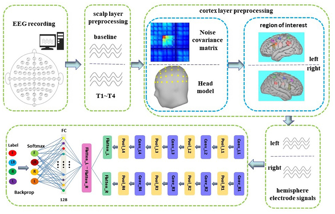
This is where deep learning (DL) has revolutionized the field. Instead of an expert hand-engineering features, a deep neural network—most commonly a Convolutional Neural Network (CNN) or a Recurrent Neural Network (RNN)—can learn the optimal features directly from the raw or minimally processed data.

This is an "end-to-end" approach where feature extraction and classification are combined into a single, trainable model.

To understand how a CNN does this, let's watch a video that explains the concept for image analysis. The core idea of hierarchical feature learning is directly transferable to time-series signals like EEG.

Now, how does this apply to EEG or other physiological signals?

• Instead of a 2D filter sliding over an image, you have a 1D filter sliding over a time-series.
• The first layer of the CNN might learn to detect simple signal shapes, like sharp peaks or basic oscillations (the "letters").
• Deeper layers would learn to combine these simple shapes into more complex, meaningful patterns relevant to the task, like a specific type of brainwave or an artifact signature (the "words" and "phrases").

This approach automates the most difficult part of the traditional pipeline and has shown state-of-the-art performance in many areas.

Conclusion

Today, we've dissected the critical roles machine learning plays in transforming noisy physiological signals into meaningful, actionable information. This pipeline is the foundation of modern biomedical instrumentation and neurotechnology.

Key Takeaways:

• The ML Pipeline: A standard workflow consists of artifact removal, feature extraction, and classification.
• Artifact Removal: ML techniques like ICA can mathematically separate clean signals from noise sources like eye blinks and muscle activity.
• Feature Extraction & Classification:
  • Traditional Approach: Experts handcraft features (e.g., HRV statistics, EEG band power) and feed them into classic classifiers like SVM or Random Forest.
  • Deep Learning Approach: Models like CNNs perform end-to-end learning, automatically discovering and classifying relevant features directly from the data.
• Trade-offs: The traditional approach is more interpretable but relies on prior knowledge. The deep learning approach is often more powerful but requires larger datasets and can be a "black box."

For your work at Neuraease, you'll need to make strategic decisions about which approach to use. You might start with a traditional pipeline using well-understood features for HRV and EDA, and later explore deep learning as you collect more data to potentially discover novel patterns predictive of emotional dysregulation.

Preview of the Next Lesson:
This was our final lesson focused on a specific component of the nervous system. As we approach the end of the course, our focus will broaden. The next lesson will integrate the concepts we've learned—from sensors and amplifiers to signal processing and machine learning—to address the learning outcome: Evaluate the design of a microprocessor-based system for a specific medical instrumentation application. We will look at how all these pieces come together in a complete, functional device.