Optimizing Large Model Training on Limited Hardware

Hello! Welcome back to our module on Efficient AI: Deployment and Optimization.

In our previous lessons, we explored how to efficiently run large, pre-trained models on local hardware using tools like llama.cpp, Ollama, and text-generation-webui. We've focused entirely on inference. Now, we pivot to the other side of the deep learning coin: training.

Training large models is far more demanding than inference, especially in terms of memory. Your learning outcome for today is to: Apply mixed-precision training and gradient accumulation for training large models on limited hardware.

These two techniques are fundamental tools in the modern ML engineer's toolkit. They are often the difference between a training job that runs successfully on your hardware and one that immediately crashes with an "out of memory" error. We will cover:

1. The Memory Bottleneck: Why training consumes so much VRAM.
2. Automatic Mixed-Precision (AMP) Training: Using lower-precision numbers to save memory and accelerate computation.
3. Gradient Accumulation: Simulating large batch sizes to improve training stability without needing more memory.
4. Combining the Techniques: Implementing a training loop that uses both methods for maximum efficiency.

Let's begin by understanding the problem we're trying to solve.

---

1. The Memory Bottleneck in Training

Why is training so much more memory-intensive than inference? During inference, a model's weights are loaded, and a forward pass is computed. During training, however, the GPU must store several large tensors in memory.

As the video explains, the total memory consumption during training is dominated by four main components:

1. Model Parameters (Weights): This is the core of your model. For a model with $N$ parameters, this requires $4N$ bytes in standard 32-bit floating-point (FP32) precision.
2. Gradients: During backpropagation, we compute a gradient for each parameter. These gradients are the same size as the parameters, adding another $4N$ bytes.
3. Optimizer States: Modern optimizers like Adam store additional information to guide the training process. Adam, for instance, stores the first moment (momentum) and second moment (variance) for each parameter. In FP32, this adds another $4N+4N=8N$ bytes.
4. Activations: To compute gradients, we must store the intermediate outputs (activations) of each layer from the forward pass. For deep models and large batch sizes, the memory required for activations can be enormous.

Let's quantify this for a 1.5 billion parameter model using Adam, as discussed in the video:

• Parameters (FP16 copy for forward/backward pass): $1.5\times 10^9\times 2\text{ bytes}\approx 3\text{ GB}$
• Gradients (FP16): $1.5\times 10^9\times 2\text{ bytes}\approx 3\text{ GB}$
• Optimizer States (FP32 master weights, momentum, variance): $1.5\times 10^9\times (4+4+4)\text{ bytes}\approx 18\text{ GB}$
• Activations: Highly dependent on architecture, sequence length, and batch size, but can easily be tens of GB.

Summing just the model and optimizer states gives us $3+3+18=24$ GB, already exceeding the VRAM of many high-end consumer GPUs, and that's before accounting for activations. This is the problem we need to solve.

---

2. Automatic Mixed-Precision (AMP) Training

Our first strategy targets the precision of our numbers. Instead of using FP32 for everything, we can use 16-bit floating-point (FP16), which halves the memory footprint and can be significantly faster on modern GPUs with specialized hardware like NVIDIA's Tensor Cores.

However, simply switching everything to FP16 is problematic.

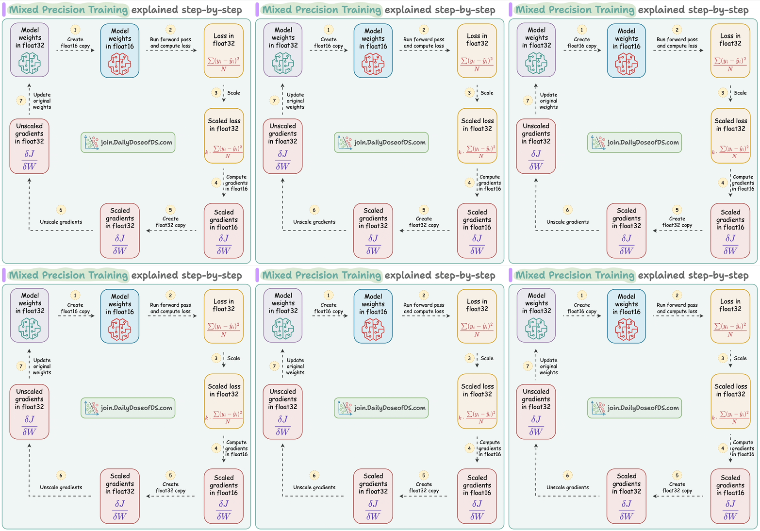
The core idea of mixed-precision training is to get the best of both worlds: use FP16 for speed and memory savings where possible, but revert to FP32 for operations that require higher precision to maintain numerical stability.

This is achieved through a three-part strategy:

1. Maintaining FP32 Master Weights: A master copy of the model's weights is kept in FP32. This ensures that small gradient updates are accumulated accurately over time.
2. Casting for Forward/Backward Pass: For each pass, a temporary FP16 copy of the weights is created. The bulk of the computation (matrix multiplications, convolutions) happens in fast FP16.
3. Loss Scaling: To prevent gradient underflow, the loss value is multiplied by a large scaling factor before backpropagation. The chain rule ensures all gradients are scaled by the same factor, shifting their values into the representable range of FP16. Before the optimizer updates the FP32 master weights, these gradients are unscaled.

Implementation in PyTorch

Manually implementing this would be complex, but PyTorch provides two utilities that make it incredibly simple: torch.amp.autocast and torch.amp.GradScaler.

Here is a typical training loop with AMP:

import torch
from torch.amp import autocast, GradScaler

# 1. Initialize the GradScaler
scaler = GradScaler()
model = ...
optimizer = ...
dataloader = ...

for batch in dataloader:
    optimizer.zero_grad()

    # 2. Wrap the forward pass with the autocast context manager
    # It automatically casts operations to FP16 where safe
    with autocast(device_type='cuda', dtype=torch.float16):
        outputs = model(batch['input'])
        loss = criterion(outputs, batch['labels'])

    # 3. Scale the loss and call backward() on the scaled loss
    scaler.scale(loss).backward()

    # 4. scaler.step() first unscales the gradients of the optimizer's params.
    # If no infs or NaNs are found, it calls optimizer.step().
    # Otherwise, optimizer.step() is skipped.
    scaler.step(optimizer)

    # 5. Update the scale for the next iteration.
    scaler.update()

This simple structure allows you to reap the benefits of mixed-precision training with minimal code changes.

---

3. Gradient Accumulation

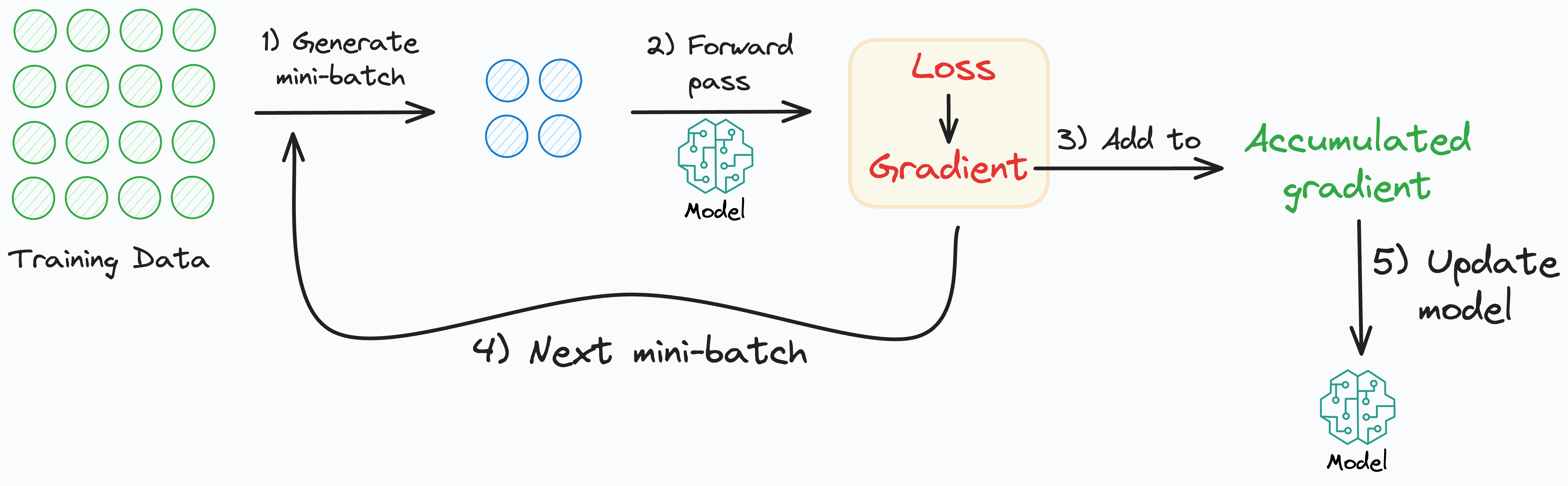
AMP helps, but you might still be unable to fit a sufficiently large batch size into memory. Small batch sizes can lead to noisy gradients and unstable training. Gradient accumulation is a clever trick to simulate a larger "virtual" batch size.

The idea is to process several smaller mini-batches sequentially, summing (accumulating) their gradients, and only performing the model weight update after a specified number of steps.

Implementation in PyTorch

The implementation relies on the fact that calls to .backward() sum up gradients in the .grad attribute of tensors. You only clear them when you call optimizer.zero_grad().

# Desired "virtual" batch size = 64
# GPU can only handle a mini-batch size of 16
mini_batch_size = 16
accumulation_steps = 4 # 16 * 4 = 64

model = ...
optimizer = ...
dataloader = ... # with batch_size=mini_batch_size

for i, batch in enumerate(dataloader):
    # Forward pass
    outputs = model(batch['input'])
    loss = criterion(outputs, batch['labels'])

    # Normalize the loss
    # Since we are summing gradients from `accumulation_steps` batches,
    # we should average the loss over them.
    loss = loss / accumulation_steps

    # Backward pass to accumulate gradients
    loss.backward()

    # Perform a weight update every `accumulation_steps`
    if (i + 1) % accumulation_steps == 0:
        optimizer.step()      # Update weights
        optimizer.zero_grad() # Reset gradients for the next accumulation cycle

The crucial detail here is dividing the loss by accumulation_steps. This ensures that the magnitude of the accumulated gradient is equivalent to what it would have been for a single large batch, rather than being accumulation_steps times larger.

Test your understanding!

You want an effective batch size of 256. Your GPU can only handle a maximum batch size of 8. What value should you set for accumulation_steps?

Show answer

You should set accumulation_steps to 32. The effective batch size is calculated as mini_batch_size * accumulation_steps. In this case, $8\times 32=256$.

---

4. Putting It All Together

The true power comes from combining these two techniques. You can use AMP to reduce the memory of each mini-batch, and then use gradient accumulation to reach a large, stable effective batch size.

Here is the combined code structure, which you should now be able to understand fully:

import torch
from torch.amp import autocast, GradScaler

# -- Configuration --
accumulation_steps = 4
model = ...
optimizer = ...
dataloader = ...

# -- Initialization --
scaler = GradScaler()
model.train()
optimizer.zero_grad()

# -- Training Loop --
for step, batch in enumerate(dataloader):
    # Use autocast for the forward pass
    with autocast(device_type='cuda', dtype=torch.float16):
        outputs = model(batch['input'])
        loss = criterion(outputs, batch['labels'])
        
        # Normalize loss for accumulation
        loss = loss / accumulation_steps

    # scaler.scale().backward() accumulates scaled gradients
    scaler.scale(loss).backward()

    # Update weights and reset gradients every accumulation_steps
    if (step + 1) % accumulation_steps == 0:
        scaler.step(optimizer)
        scaler.update()
        optimizer.zero_grad()

This combined pattern is a standard and highly effective way to train large models on hardware with limited VRAM.

---

Conclusion

In this lesson, you've learned two indispensable techniques for efficient model training. These methods move beyond pure theory and into the practical engineering required to work with state-of-the-art models.

Key Takeaways:

• Training Memory: Is dominated by model parameters, gradients, optimizer states, and activations.
• Automatic Mixed-Precision (AMP): Reduces memory usage and leverages specialized hardware by performing computations in FP16, while maintaining numerical stability with FP32 master weights and loss scaling.
• Gradient Accumulation: Simulates a larger batch size by accumulating gradients over several mini-batches before updating model weights, leading to more stable training on memory-constrained hardware.
• Combined Approach: Using AMP and gradient accumulation together is a powerful and standard strategy for training large models on consumer-grade GPUs.

Preview of the Next Lesson:

We've successfully optimized training on a single GPU. But what if one GPU isn't enough, no matter how much we optimize? The next step in scaling is to distribute the workload across multiple GPUs or even multiple machines. In the next lesson, you will learn to "Implement distributed training strategies like Data Parallelism and Pipeline Parallelism", which are the techniques used to train truly massive models like GPT-3 and Llama.