Distributed Training Strategies

Hello! Welcome to the final lesson in our module on Efficient AI: Deployment and Optimization.

In our last session, we focused on squeezing the most out of a single GPU by using mixed-precision training and gradient accumulation. These are powerful tools, but they have their limits. What happens when a model is simply too large to fit in one GPU's memory, or when training on one GPU is too slow, even with optimizations? To overcome these barriers, we must scale out.

This lesson addresses your final learning outcome for this module: to implement distributed training strategies like Data Parallelism and Pipeline Parallelism. We will explore how to harness the power of multiple GPUs—and even multiple machines—to train models at a scale that would otherwise be impossible.

We will cover:

1. The Two Fundamental Approaches: An overview of Data Parallelism vs. Model Parallelism.
2. Data Parallelism: How to replicate a model to process data faster, and how to implement it with PyTorch's DistributedDataParallel (DDP).
3. Pipeline Parallelism: A smart form of model parallelism that splits the model across GPUs and uses micro-batching to keep them all busy.
4. Combining Strategies: A look at how state-of-the-art training setups mix and match different parallelism techniques for maximum efficiency.

Let's begin our journey into large-scale distributed training.

---

1. Scaling Up: Two Parallel Paths

When you have more than one GPU, there are two fundamental ways to distribute the training workload:

• Data Parallelism: You have one model, but a lot of data. So, you replicate the model on each GPU and give each replica a different slice of the data to process. This is like hiring multiple identical workers to each work on a different part of a large project. The primary goal is to increase throughput and reduce training time.
• Model Parallelism: You have one model that is too large to fit on a single GPU. So, you split the model itself across multiple GPUs, with each GPU holding a different piece. This is like having a team of specialized workers, each responsible for one stage of an assembly line. The primary goal is to overcome memory limitations.

We will explore the most common and effective implementations of both approaches.

---

2. Data Parallelism: Replicate and Conquer

Data Parallelism is the most common and often the simplest strategy to implement. The core idea is straightforward: if one GPU can process a batch of 32 in one second, four GPUs should be able to process a batch of 128 in roughly the same amount of time.

How Data Parallelism Works

The process involves a synchronized dance between the GPUs, orchestrated by communication primitives.

To summarize the key steps of a DistributedDataParallel (DDP) training iteration:

1. Setup: The model is initialized on one GPU (the rank 0 process) and its weights are broadcast to all other GPUs. Now, every GPU has an identical copy of the model.
2. Data Sharding: The global data batch is split, and each GPU receives its own mini-batch.
3. Local Computation: Each GPU independently performs a forward and backward pass on its mini-batch, calculating local gradients. At this point, each GPU has different gradients because they processed different data.
4. Gradient Synchronization: This is the magic of DDP. The gradients from all GPUs are averaged together using an all-reduce operation. This operation efficiently sums all the gradients and distributes the result (the average) back to all GPUs.
5. Weight Update: Each GPU's optimizer updates its local model copy using the identical, averaged gradients. Because they all start with the same weights and apply the same update, the model replicas remain perfectly synchronized.

This process repeats for each batch, effectively parallelizing the computation across GPUs while ensuring the model learns consistently.

Implementation with PyTorch DDP

PyTorch's torch.nn.parallel.DistributedDataParallel module makes implementing this strategy surprisingly manageable. The changes are mostly boilerplate code around your existing training loop.

Here is a summary of the key modifications to a standard training script:

import torch
import torch.distributed as dist
from torch.nn.parallel import DistributedDataParallel as DDP
from torch.utils.data import DataLoader
from torch.utils.data.distributed import DistributedSampler
import os

def setup(rank, world_size):
    # These environment variables are set by torchrun
    os.environ['MASTER_ADDR'] = 'localhost'
    os.environ['MASTER_PORT'] = '12355'
    # Initialize the process group
    dist.init_process_group("nccl", rank=rank, world_size=world_size)

def cleanup():
    dist.destroy_process_group()

def train(rank, world_size):
    setup(rank, world_size)
    
    # Create model and move it to the correct GPU
    model = YourModel().to(rank)
    # Wrap the model with DDP
    ddp_model = DDP(model, device_ids=[rank])

    # Use DistributedSampler to handle data sharding
    dataset = YourDataset()
    sampler = DistributedSampler(dataset, num_replicas=world_size, rank=rank)
    dataloader = DataLoader(dataset, batch_size=..., sampler=sampler)

    optimizer = torch.optim.SGD(ddp_model.parameters(), lr=0.001)

    for epoch in range(num_epochs):
        # The sampler needs the epoch to shuffle data properly
        sampler.set_epoch(epoch)
        for batch in dataloader:
            inputs, labels = batch
            inputs, labels = inputs.to(rank), labels.to(rank)
            
            optimizer.zero_grad()
            outputs = ddp_model(inputs)
            loss = loss_fn(outputs, labels)
            loss.backward() # DDP handles the all-reduce automatically here
            optimizer.step()

    cleanup()

# To run this code for 4 GPUs, you would use the command line:
# torchrun --nproc_per_node=4 your_script.py

The main drawback of data parallelism is clear: each GPU must hold a full copy of the model, its gradients, and its optimizer states. It solves the speed problem but not the memory problem.

---

3. Pipeline Parallelism: The Assembly Line for Models

What if your model is so large it doesn't fit on a single GPU? This is where Model Parallelism comes in. The simplest form is to just place different layers on different GPUs.

However, this naive approach is highly inefficient.

Pipeline Parallelism refines naive model parallelism into an efficient strategy. Here’s how it works:

1. Partition the Model: The model is split into several sequential "stages." Each stage (a group of layers) is placed on a different GPU.
2. Split the Batch: The data batch is split into multiple smaller micro-batches.
3. Pipeline Execution:
   • GPU 0 processes the first micro-batch and passes its output to GPU 1.
   • As GPU 1 works on the first micro-batch, GPU 0 immediately starts processing the second micro-batch.
   • This continues down the line, creating a "pipeline" of micro-batches flowing through the model stages. This ensures that, after a brief startup period, all GPUs are working in parallel on different micro-batches.

The backward pass works similarly, with gradients flowing back up the pipeline.

Implementation and Trade-offs

Manually implementing pipeline parallelism is complex, involving careful management of tensor transfers and synchronization. Frameworks like DeepSpeed and Megatron-LM automate this. The concept, however, is key.

The key advantage is enabling the training of massive models. The main disadvantage is the implementation complexity and the unavoidable "pipeline bubble" at the start and end of processing a batch, where not all GPUs are active.

Test your understanding!

You are training a model with 12 layers on 4 GPUs using pipeline parallelism. You split the model into 4 stages, with 3 layers per stage. In a naive model-parallel setup (without pipelining), how many GPUs are active at any given moment during the forward pass for a single data sample? How does pipeline parallelism with micro-batching change this?

Show answer

In a naive model-parallel setup, only one GPU is active at any time. GPU 0 processes layers 1-3, then GPU 1 processes layers 4-6, and so on. The other three GPUs are idle.

With pipeline parallelism, after an initial "fill" period, all four GPUs can be active simultaneously, each working on a different micro-batch at a different stage of the model. This dramatically improves overall hardware utilization.

---

4. Combining Strategies for Maximum Scale

Data Parallelism and Pipeline Parallelism are not mutually exclusive. In fact, training state-of-the-art large language models almost always involves combining multiple parallelism strategies to balance memory, compute, and communication overhead.

This is often called 2D or 3D Parallelism.

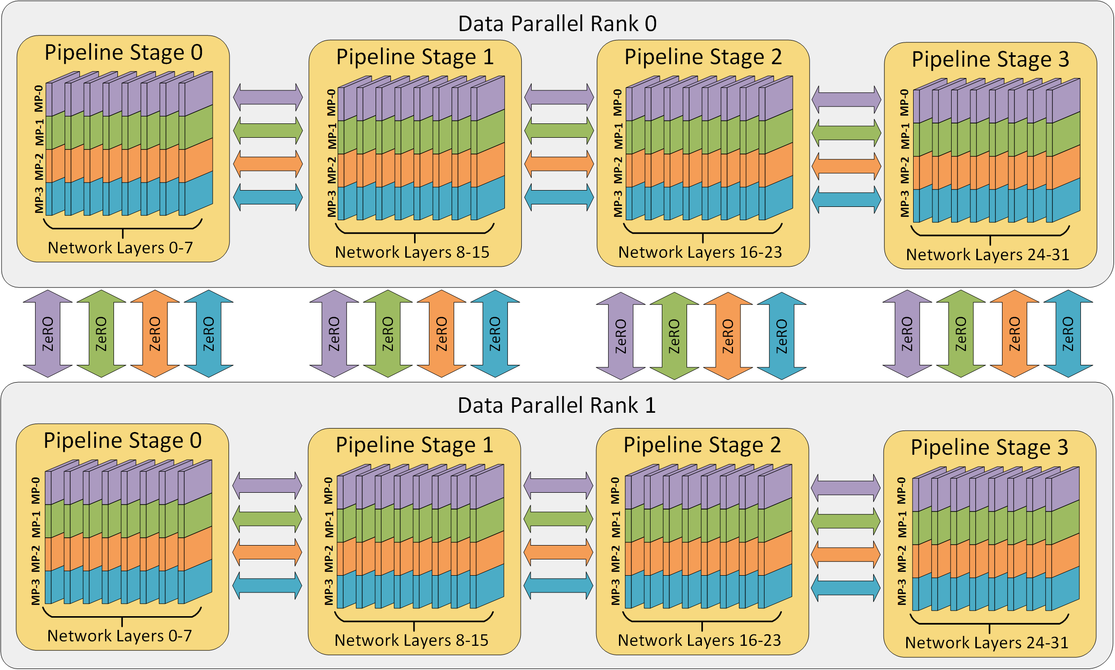
A common and powerful hybrid strategy is Data + Pipeline Parallelism:

• You first split your huge model across several GPUs using Pipeline Parallelism. This group of GPUs forms one "replica" of the model.
• Then, you create multiple such replicas and use Data Parallelism to feed different data batches to each replica.

This allows you to scale both the model size (with PP) and the data throughput (with DP) simultaneously. The image shown earlier (3d-parallelism.png) depicts exactly this: two "Data Parallel Ranks," where each rank is a 4-stage pipeline.

---

Conclusion

You have now completed our module on efficient AI! We've journeyed from optimizing for a single GPU to orchestrating a fleet of them for large-scale training.

Key Takeaways:

• Distributed training addresses two bottlenecks: compute speed (training time) and memory capacity.
• Data Parallelism (DDP) is the go-to strategy for speeding up training when your model fits on a single GPU. It replicates the model, shards the data, and uses all-reduce to sync gradients.
• Pipeline Parallelism (PP) is a form of model parallelism that enables training of models too large for one GPU. It splits the model into stages and uses micro-batching to keep all GPUs utilized.
• Hybrid Strategies are the standard for SOTA training, combining Data, Pipeline, and other forms of parallelism (like Tensor Parallelism) to create powerful 2D and 3D training configurations.

Preview of the Next Module:

We have now covered the fundamental algorithms, architectures (MLPs, CNNs, RNNs, Transformers), and training techniques that power modern AI. With this foundation, we are ready to look at the absolute cutting edge. In our next module, "Emerging Architectures and Research Frontiers," we will begin by exploring architectures that challenge the Transformer's dominance, starting with State Space Models like Mamba.