Wav2Vec 2.0 Architecture: Encoder and Transformer

Hello! Welcome to your second lesson in the "Self-Supervised Speech Representation" module.

In our last lesson, we explored the motivation for self-supervised learning (SSL). We established that the reliance on vast amounts of labeled data is a major bottleneck in speech processing and that SSL, inspired by models like BERT in NLP, offers a path to leverage abundant unlabeled audio. We ended by highlighting the core challenge: unlike discrete text, speech is a continuous waveform, which requires a new approach to enable BERT-like masked prediction tasks.

Today, we will dissect the architecture of wav2vec 2.0, a seminal model that provides an elegant solution to this problem. This lesson directly addresses the learning outcome: Describe the wav2vec 2.0 architecture, detailing its CNN feature encoder and Transformer context network. We will break down the model into its two primary components, understanding the specific role each one plays in transforming a raw audio signal into rich, contextualized representations.

1. The Wav2vec 2.0 Architectural Blueprint

At its core, wav2vec 2.0 is designed to first extract local, high-level features from raw audio and then use a powerful context network to understand the relationships between these features across an entire utterance. This dual-component design is a common pattern in modern speech models.

Let's begin with a high-level overview of the data flow.

As the video illustrates, the architecture consists of three main parts:

1. A CNN-based Feature Encoder that processes the raw audio waveform.
2. A Quantization Module that discretizes the output of the feature encoder.
3. A Transformer-based Context Network that builds the final representations.

In this lesson, we will focus on #1 and #3. We'll examine the quantization module and the training objective in detail in our next session.

2. The Feature Encoder: From Waveform to Latent Features

The first challenge is to process the raw audio waveform, which can have a high sampling rate (e.g., 16,000 samples per second), into a more manageable sequence of feature vectors. This is the job of the feature encoder. Instead of using traditional hand-crafted features like MFCCs, wav2vec 2.0 uses a neural network to learn the optimal features directly from the data.

This feature encoder is a multi-layer 1D Convolutional Neural Network (CNN). Its primary functions are:

• Feature Extraction: It learns to extract meaningful acoustic features from short segments of the raw audio.
• Downsampling: Through strided convolutions, it reduces the temporal resolution of the signal. A 16kHz audio signal is transformed into a sequence of feature vectors where each vector represents approximately 20ms of audio. This is conceptually similar to the frame-based analysis used in STFT.

Let's look at a more detailed diagram of this component.

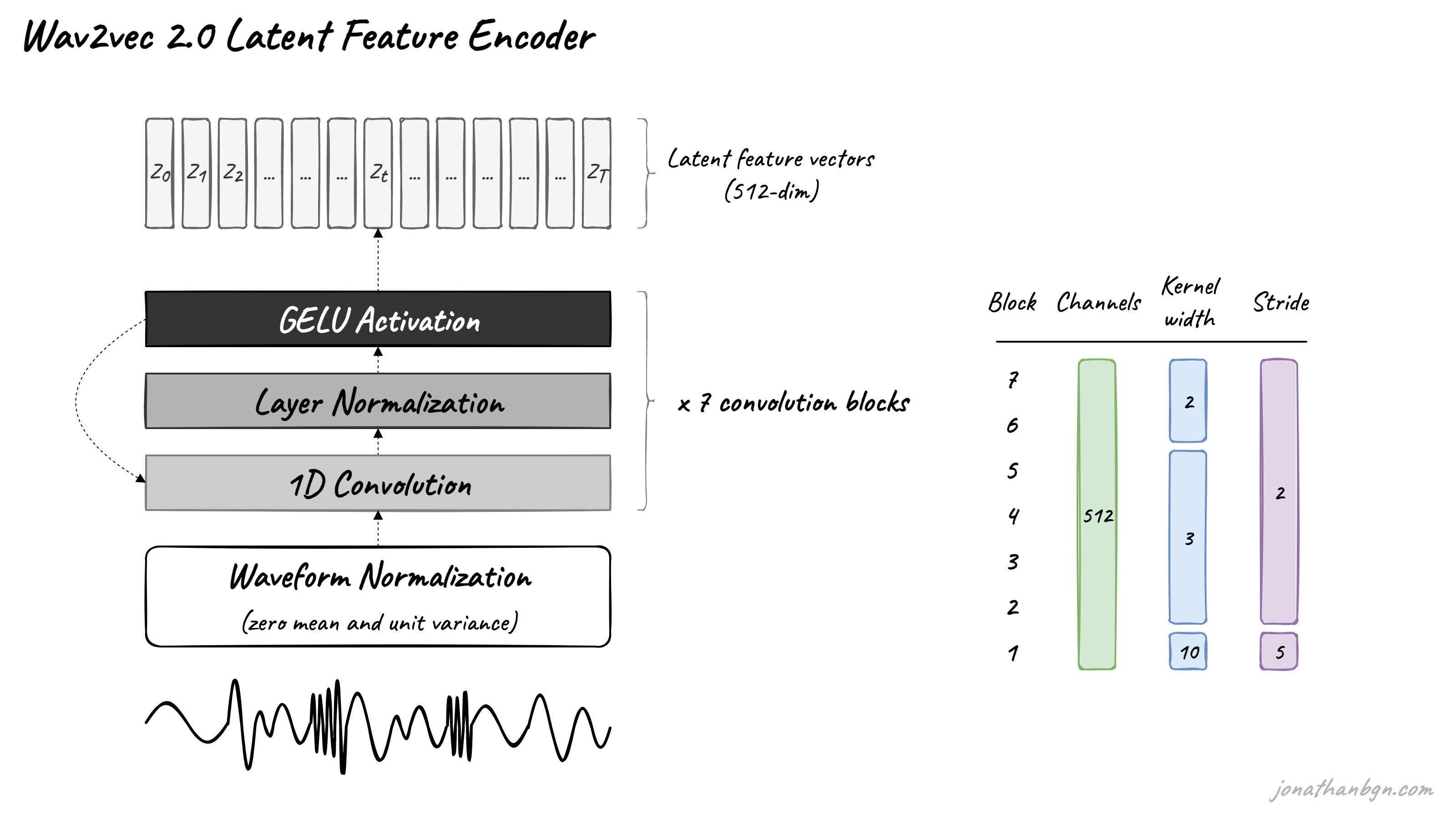
The key characteristics of this encoder are:

• Input: A 1D tensor representing the normalized raw audio waveform, $X$.
• Architecture: Seven layers of 1D convolutions with 512 channels. The kernel sizes and strides are designed to have a total receptive field of 25ms (400 samples at 16kHz).
• Activation: The GELU (Gaussian Error Linear Unit) activation function is used, which is common in Transformer-based models.
• Output: A sequence of latent feature vectors $Z=[z_1,z_2,...,z_T]$, where each $z_t$ is a 512-dimensional vector. The sequence length $T$ is significantly shorter than the original waveform length due to the strided convolutions.

This process $f:X\to Z$ gives us a sequence of rich, locally-aware feature vectors that are ready to be processed for global context.

3. The Context Network: Building Global Understanding

Once we have the sequence of local feature vectors $Z$, we need to understand the long-range dependencies between them. A feature vector representing the phoneme /k/ is ambiguous on its own; its meaning is clarified by the surrounding sounds that form a word. This is where the Transformer comes in.

The context network in wav2vec 2.0 is a standard Transformer encoder. It takes the sequence of latent features $Z$ and produces a new sequence of contextualized representations $C$.

The key characteristics of the context network are:

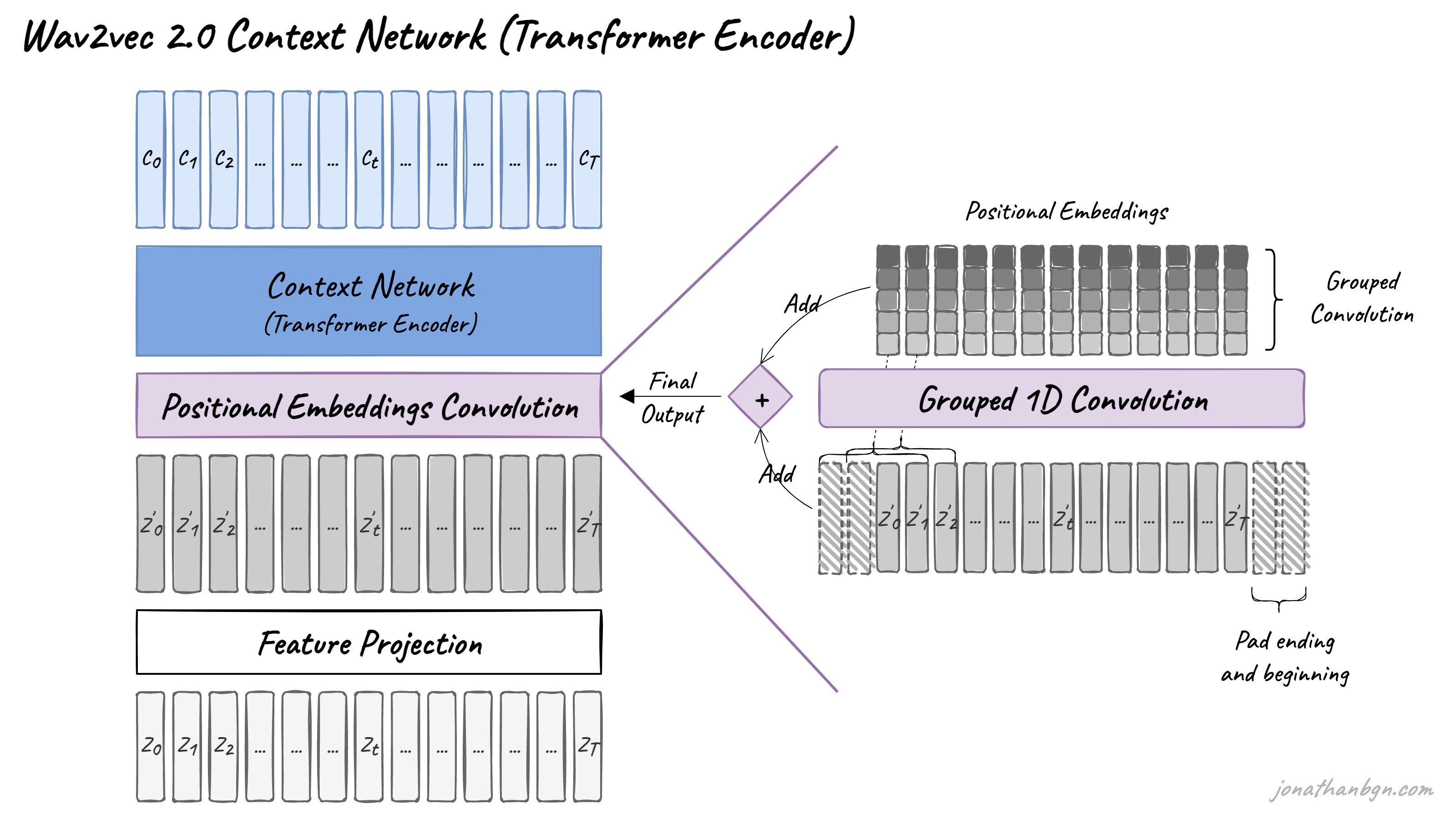
• Input: The sequence of latent representations $Z$. Before being fed to the Transformer, these 512-dim vectors are passed through a linear projection layer to match the Transformer's internal dimension (768 for BASE, 1024 for LARGE).
• Architecture: A stack of Transformer encoder blocks. The BASE model uses 12 blocks, and the LARGE model uses 24. Each block consists of a multi-head self-attention layer followed by a feed-forward network, with residual connections and layer normalization.
• Output: A sequence of context vectors $C=[c_1,c_2,...,c_T]$, where each $c_t$ has encoded information from the entire input sequence.

A Special Note on Positional Embeddings

A crucial detail, especially given your familiarity with Transformers, is how wav2vec 2.0 handles positional information. The original Transformer added fixed sinusoidal positional embeddings to its input. Wav2vec 2.0 takes a different approach. It uses a small, lightweight 1D convolution layer that is applied to the latent features $Z$ before they enter the main Transformer stack. The output of this convolutional layer is then added to the feature vectors, effectively injecting relative positional information. This allows the model to learn its own positional embeddings dynamically.

This entire process $g:Z\to C$ mirrors the function of BERT, but operates on learned acoustic features instead of text embeddings.

Summary: The Complete Architectural Flow

Let's put everything together. The wav2vec 2.0 architecture processes speech as follows:

1. Input: A raw audio waveform $X$ is fed into the model.
2. Local Feature Extraction: The CNN Feature Encoder acts as a learned front-end, processing the waveform to produce a sequence of local, latent representations $Z$. This step reduces dimensionality and extracts key acoustic patterns. $$Z=\text{CNN}(X)$$
3. Contextualization: Before entering the Transformer, some timesteps of $Z$ are masked. The Transformer Context Network then processes this masked sequence, and its self-attention mechanism allows each timestep to gather information from all other timesteps, producing the final contextual representations $C$. $$C=\text{Transformer}(\text{Mask}(Z))$$

The model is then trained to use the output $c_t$ at a masked timestep $t$ to identify the original, unmasked latent feature $z_t$. This forces the context network to learn powerful representations that capture both phonetic content and long-term contextual dependencies.

For a final review, you can consult this alternative explanation which consolidates these concepts.

Conclusion

In this lesson, we have dissected the two core components of the wav2vec 2.0 architecture. You now understand how it leverages a combination of convolutional and Transformer layers to create powerful representations directly from raw audio.

Key Takeaways:

• Dual-Component Architecture: wav2vec 2.0 uses a CNN feature encoder for local feature extraction and a Transformer context network for global context modeling.
• CNN Feature Encoder: It takes a raw waveform as input and outputs a sequence of lower-resolution, 512-dimensional latent feature vectors ($Z$), effectively acting as a learned replacement for traditional features like MFCCs.
• Transformer Context Network: It processes the sequence of latent features to produce contextualized representations ($C$), where each output vector contains information from the entire sequence. It uses a novel convolutional approach for relative positional embeddings.
• Data Flow: The overall flow is $X\stackrel{\text{CNN}}{\to }Z\stackrel{\text{Transformer}}{\to }C$, with a masking step applied to $Z$ before it enters the Transformer.

Preview of the Next Lesson:

We've focused on the "what" and "how" of the architecture. The next crucial question is: how does the model actually learn during the pre-training phase? In the next lesson, we will dive into the wav2vec 2.0 pretraining objective. We'll explore the ingenious quantization module used to create discrete targets from the continuous latent features and the contrastive loss that drives the model to learn meaningful speech representations.