Wav2Vec 2.0 Pretraining: Quantization & Contrastive Loss

Hello! Welcome to the third lesson in our "Self-Supervised Speech Representation" module.

In our previous lesson, we dissected the architecture of wav2vec 2.0, establishing how its CNN feature encoder and Transformer context network work together to transform a raw audio waveform ($X$) into a sequence of latent features ($Z$) and finally into contextualized representations ($C$). We noted that the model learns by predicting masked portions of the latent sequence, but we left a crucial question unanswered: how can a model predict targets in a continuous signal like speech, a problem not present in text-based models like BERT?

Today, we will answer that question by diving into the heart of wav2vec 2.0's learning strategy. This lesson directly addresses the learning outcome: Explain the wav2vec 2.0 pretraining objective, including the role of the quantization module and contrastive loss.

We will explore three key components:

1. The Quantization Module: An ingenious mechanism to create discrete, predictable targets from continuous speech features.
2. The Contrastive Loss: The core training objective that forces the model to learn meaningful representations by distinguishing correct targets from distractors.
3. The Diversity Loss: An auxiliary loss that acts as a regularizer to ensure the model uses its full representational capacity.

---

1. The Pre-Training Task: Masked Prediction with a Twist

The fundamental idea behind wav2vec 2.0's pre-training is inspired by Masked Language Modeling (MLM) in BERT. The model masks certain parts of the input sequence and is tasked with predicting the original content of the masked parts.

However, there's a critical difference. BERT deals with discrete tokens (words or subwords) from a finite vocabulary. The latent features $Z$ produced by wav2vec 2.0's encoder are continuous-valued vectors. Directly trying to predict these continuous vectors (e.g., via regression) poses two problems:

• It's an unstable and difficult learning task.
• The model might learn trivial solutions, like simply encoding speaker identity or background noise, rather than the underlying phonetic content, which is more useful for downstream tasks like ASR.

The solution is to discretize the continuous latent representations into a finite set of discrete "acoustic units." These discrete units then serve as the targets for the prediction task. This is the primary function of the quantization module.

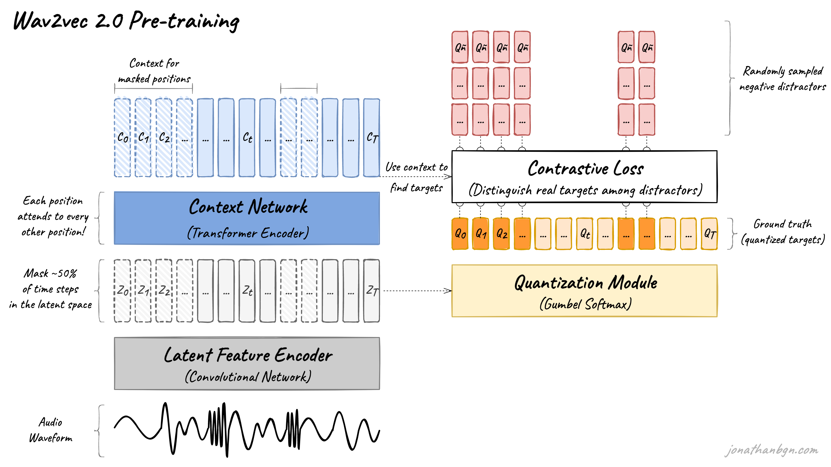
Let's start with a visual overview of this entire pre-training setup.

---

2. The Quantization Module: Forging Discrete Targets

The quantization module's job is to convert each continuous latent vector $z_t$ into a discrete, quantized vector $q_t$.

A simple way to do this would be to use a single, large codebook of vectors (like a dictionary) and find the closest entry for each $z_t$. However, this is computationally inefficient. Wav2vec 2.0 employs a more sophisticated method called Product Quantization.

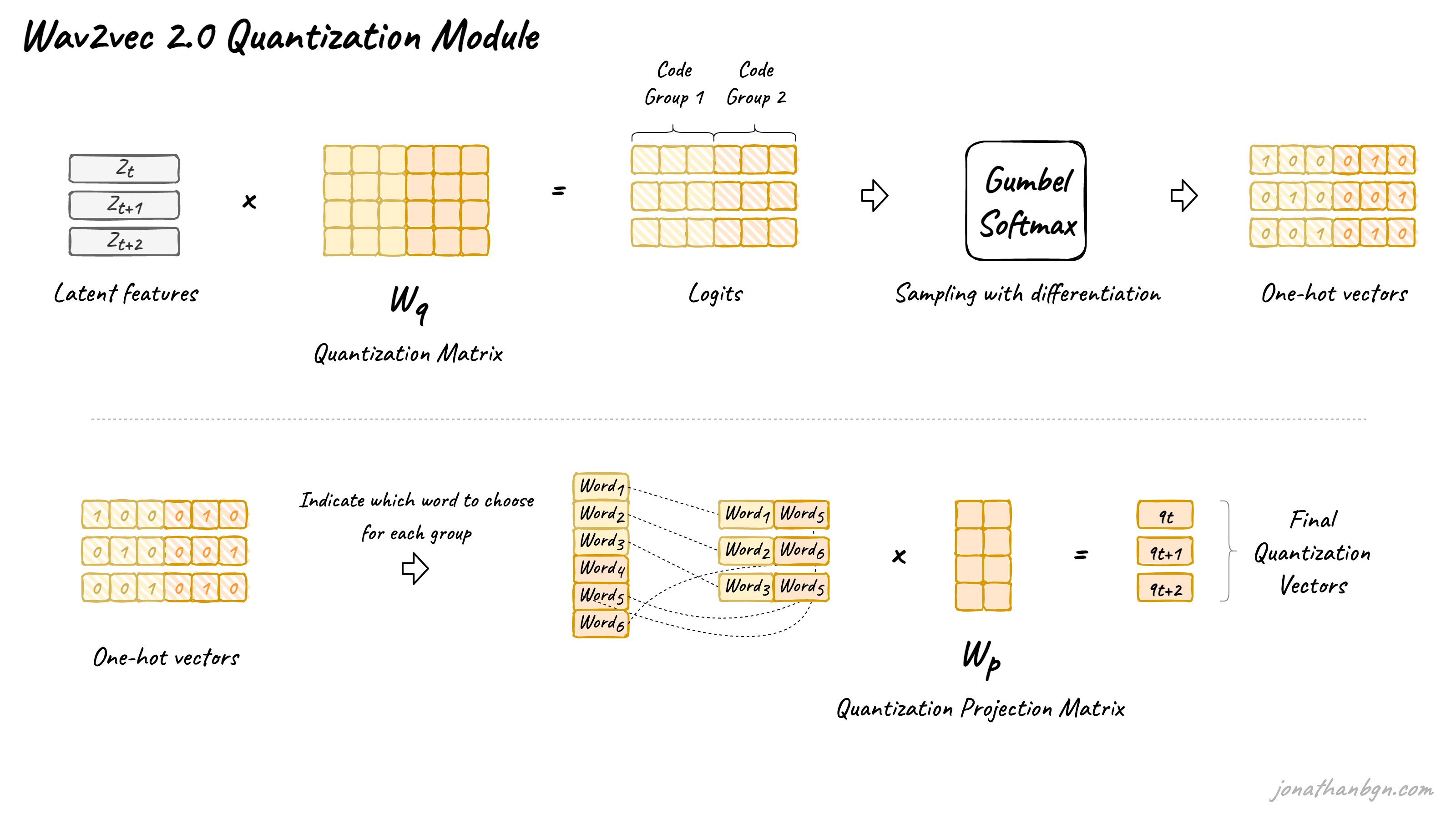
• Product Quantization: Instead of one large codebook, it uses $G$ smaller codebooks (called groups), each containing $V$ vector entries. To quantize a vector, it selects one entry from each of the $G$ codebooks, concatenates them, and applies a linear transformation to get the final quantized vector $q_t$. For wav2vec 2.0, $G=2$ and $V=320$, allowing for $320\times 320=102,400$ possible representations.

The main challenge here is that the selection process—choosing the "best" entry from a codebook—is an argmax operation, which is not differentiable and thus breaks the backpropagation of gradients.

The Gumbel-Softmax Trick

To overcome this, wav2vec 2.0 uses the Gumbel-Softmax trick. This is a technique for drawing samples from a categorical distribution in a differentiable way, and you'll find it used in other advanced models like discrete Variational Autoencoders (VAEs).

The intuition is to create a "soft," differentiable approximation of argmax. This is done by:

1. Predicting logits (unnormalized log-probabilities) for each entry in a codebook.
2. Adding random noise drawn from a Gumbel distribution to these logits.
3. Applying a softmax function with a temperature parameter $\tau$.

The resulting equation for the probability of choosing the $v$-th codebook entry for group $g$ is:

$$p_{g,v}=\frac{\exp ((l_{g,v}+n_v)/\tau )}{{\sum }_{k=1}^V\exp ((l_{g,k}+n_k)/\tau )}$$

where $l_{g,v}$ is the logit, $n_v$ is the Gumbel noise, and $\tau$ is the temperature. As $\tau \to 0$, this operation becomes equivalent to an argmax. During training, this allows gradients to flow back through the selection process, while in the forward pass, a hard argmax is often used (a method known as a straight-through estimator).

This next video provides a deep dive into the quantization module and the Gumbel-Softmax trick. Given your background, the level of mathematical detail here should be particularly insightful.

This diagram provides a clear visual of the quantization process for a single group.

---

3. The Contrastive Loss ($L_m$)

Now that we have a sequence of contextualized vectors $C$ and a corresponding sequence of quantized target vectors $Q$, we can define the core training objective.

For each masked timestep $t$, the model's task is to use its contextualized output $c_t$ to identify the correct quantized target $q_t$ from a set of $K+1$ candidates. This set contains the true target $q_t$ and $K$ distractors, which are other quantized vectors randomly sampled from different masked timesteps within the same utterance.

This is framed as a contrastive task. The loss function is designed to pull the representation $c_t$ closer to the true target $q_t$ and push it away from all the distractor targets.

The loss is defined as:

$$L_m=-\log \frac{\exp (\text{sim}(c_t,q_t)/\kappa )}{{\sum }_{\tilde{q}\in Q_t}\exp (\text{sim}(c_t,\tilde{q})/\kappa )}$$

Let's break this down:

• $\text{sim}(a,b)$ is the cosine similarity between two vectors.
• $\kappa$ is a temperature parameter that sharpens the distribution, making the task more challenging.
• The overall structure is a cross-entropy loss. The numerator represents the "score" for the correct target, and the denominator is the sum of scores for all candidates (the correct one plus the distractors).
• By minimizing this loss, the model learns to produce a $c_t$ that has the highest cosine similarity with the correct $q_t$.

To solidify your understanding of this loss function, please review the following video segment and the original paper.

---

4. The Diversity Loss ($L_d$)

There's a potential failure mode in this setup known as codebook collapse. The model might find it easy to only ever use a small subset of the available codebook entries, which would limit the richness of the learned representations.

To counteract this, wav2vec 2.0 includes a diversity loss. This is an auxiliary loss that encourages the model to use all the entries in its codebooks with roughly equal frequency.

It achieves this by maximizing the entropy of the averaged probability distribution over the codebook entries across a batch of training examples. A uniform distribution has the maximum possible entropy. The loss is therefore the negative entropy, which the model seeks to minimize.

The diversity loss is formulated as:

$$L_d=\frac{1}{GV}\sum _{g=1}^G-H({\bar{p}}_g)=\frac{1}{GV}\sum _{g=1}^G\sum _{v=1}^V{\bar{p}}_{g,v}\log {\bar{p}}_{g,v}$$

where ${\bar{p}}_g$ is the averaged probability distribution for codebook $g$ across the batch.

---

5. The Final Objective and a Critical Insight

The final pre-training objective is a weighted sum of the contrastive loss and the diversity loss:

$$L=L_m+\alpha L_d$$

where $\alpha$ is a hyperparameter that balances the two terms.

An important design choice is that the Transformer context network operates on the continuous latent features $Z$, while the contrastive targets are the quantized features $Q$. Why? The paper provides a compelling ablation study.

This finding is a cornerstone of the model's success. The continuous representations fed into the Transformer retain rich, nuanced information, while the discrete, quantized targets force the model to learn more general and robust representations by abstracting away utterance-specific details like speaker voice or background noise.

---

Conclusion

In this lesson, we have unpacked the powerful pre-training objective of wav2vec 2.0. You now understand the complete process by which the model learns rich speech representations from unlabeled audio.

Key Takeaways:

• Objective: The model learns via a masked prediction task, similar to BERT. To handle continuous audio, it first discretizes the features.
• Quantization Module: This module converts continuous latent features ($z_t$) into discrete quantized targets ($q_t$) using product quantization. It uses the Gumbel-Softmax trick to make the codebook selection process differentiable.
• Contrastive Loss: This is the primary learning signal. It trains the model to identify the correct quantized target for a masked position from a set of distractors, based on the contextualized output.
• Diversity Loss: This auxiliary loss acts as a regularizer, encouraging the model to use all of its codebook entries to prevent codebook collapse and promote richer representations.
• Key Design: The model uses continuous features as input to the Transformer but quantized features as the prediction targets, which is critical for learning general, robust representations.

Preview of the Next Lesson:

We've now fully covered how wav2vec 2.0 is pre-trained. The next logical step is to see how we can leverage this powerful pre-trained model for a specific task. In our next lesson, we will focus on fine-tuning a pre-trained wav2vec 2.0 model for Automatic Speech Recognition (ASR) and compare its data efficiency to a model trained from scratch.