CTC Loss and Forward-Backward Algorithm

Hello!

In our last lesson, we framed Automatic Speech Recognition (ASR) as a sequence-to-sequence problem and identified the core alignment challenge. We introduced Connectionist Temporal Classification (CTC) at a high level as an elegant solution that avoids needing a pre-defined, hard alignment between audio frames and text characters. You learned that CTC works by summing the probabilities of all possible valid alignments that collapse down to the correct transcript.

Today, we will dive deep into the mathematics of that process. This lesson directly addresses the learning outcome: Derive the Connectionist Temporal Classification (CTC) loss function and its forward-backward algorithm. We will formalize the CTC objective, understand why a naive computation is infeasible, and then derive the dynamic programming algorithm that makes it work. This will give you the complete theoretical and mathematical foundation for one of ASR's most important components.

1. The CTC Objective Function

Let's start by formalizing the problem. Our acoustic model (e.g., a Transformer or RNN) processes an input audio sequence $X = [x_{1}, x_{2}, \dots, x_{T}]$ of length $T$ . At each of the $T$ time steps, it outputs a probability distribution over our vocabulary of $C$ characters, thanks to a softmax layer. Let's denote the probability of emitting character $k$ at time step $t$ as $p_{t} (k ∣ X)$ .

Our vocabulary includes all the standard characters plus a special blank token, $ϵ$ , which we introduced in the last lesson.

CTC Loss: Input to Output Sequence Alignment — This diagram illustrates the full CTC process. The RNN processes the input spectrogram, producing a probability distribution per time step. These probabilities define many possible alignments (paths), which are then collapsed to form the final output. The CTC loss considers all these valid paths. Source: Shujian's Blog.

An alignment, or path, $π$ , is a sequence of tokens of length $T$ , e.g., $π = [π_{1}, π_{2}, \dots, π_{T}]$ . Since the model's outputs at each time step are conditionally independent (given the input $X$ ), the probability of a specific path $π$ is simply the product of the probabilities at each step:

p (π ∣ X) = t = 1 \prod T p_{t} (π_{t} ∣ X)

As we discussed, a many-to-one mapping function, $B$ , collapses a path $π$ into the final output sequence $Y$ by first merging consecutive repeated characters and then removing all blank tokens.

The core idea of CTC is that the total probability of an output sequence $Y$ is the sum of the probabilities of all possible paths $π$ that collapse to $Y$ :

p (Y ∣ X) = π \in B^{- 1} (Y) \sum p (π ∣ X)

where $B^{- 1} (Y)$ is the set of all valid paths that map to $Y$ . The CTC loss for a given $(X, Y)$ pair is then simply the negative log-likelihood of this probability:

L_{CTC} = - lo g p (Y ∣ X)

2. The Challenge: An Intractable Sum

The objective function seems straightforward, but there's a major computational hurdle. The number of possible paths that can collapse to $Y$ is enormous and grows exponentially with the length of the input and output sequences.

Sequence Modeling with CTC

The Distill.pub article "Sequence Modeling with CTC", which you saw previously, provides an excellent, concise explanation of this computational challenge.

Please read the first three paragraphs of the "Loss Function" section, and then the first three paragraphs of the main body of section 2. Focus on the explanation of why a straightforward approach is too slow and how the insight of merging paths at the same output and step leads to a dynamic programming solution.

As the article explains, a naive summation is computationally infeasible. We need a more efficient method. The key insight is that many different paths can converge to the same state at the same time step. Instead of tracking every individual path, we can merge them and only track the total probability of reaching a certain point. This is the perfect scenario for a dynamic programming approach.

3. The Forward-Backward Algorithm

The algorithm used to efficiently compute the CTC loss is a dynamic programming technique known as the forward-backward algorithm. We will focus first on the forward pass, which is sufficient to calculate the total loss. The backward pass becomes necessary when calculating the gradients for training.

3.1. Setting up the Trellis

To simplify the algorithm, we first modify the target sequence $Y$ . For a sequence like $Y = "cat"$ , we create an expanded sequence, let's call it $Z$ , by inserting blank tokens at the beginning, at the end, and between each character:

$Z = [ϵ, c, ϵ, a, ϵ, t, ϵ]$

The length of this new sequence $Z$ is $S = 2∣ Y ∣ + 1$ . This structure helps us define a consistent set of transition rules.

We can visualize the problem as finding paths through a grid, or trellis, of size $S \times T$ . The rows correspond to the characters in $Z$ , and the columns correspond to the time steps of the audio input.

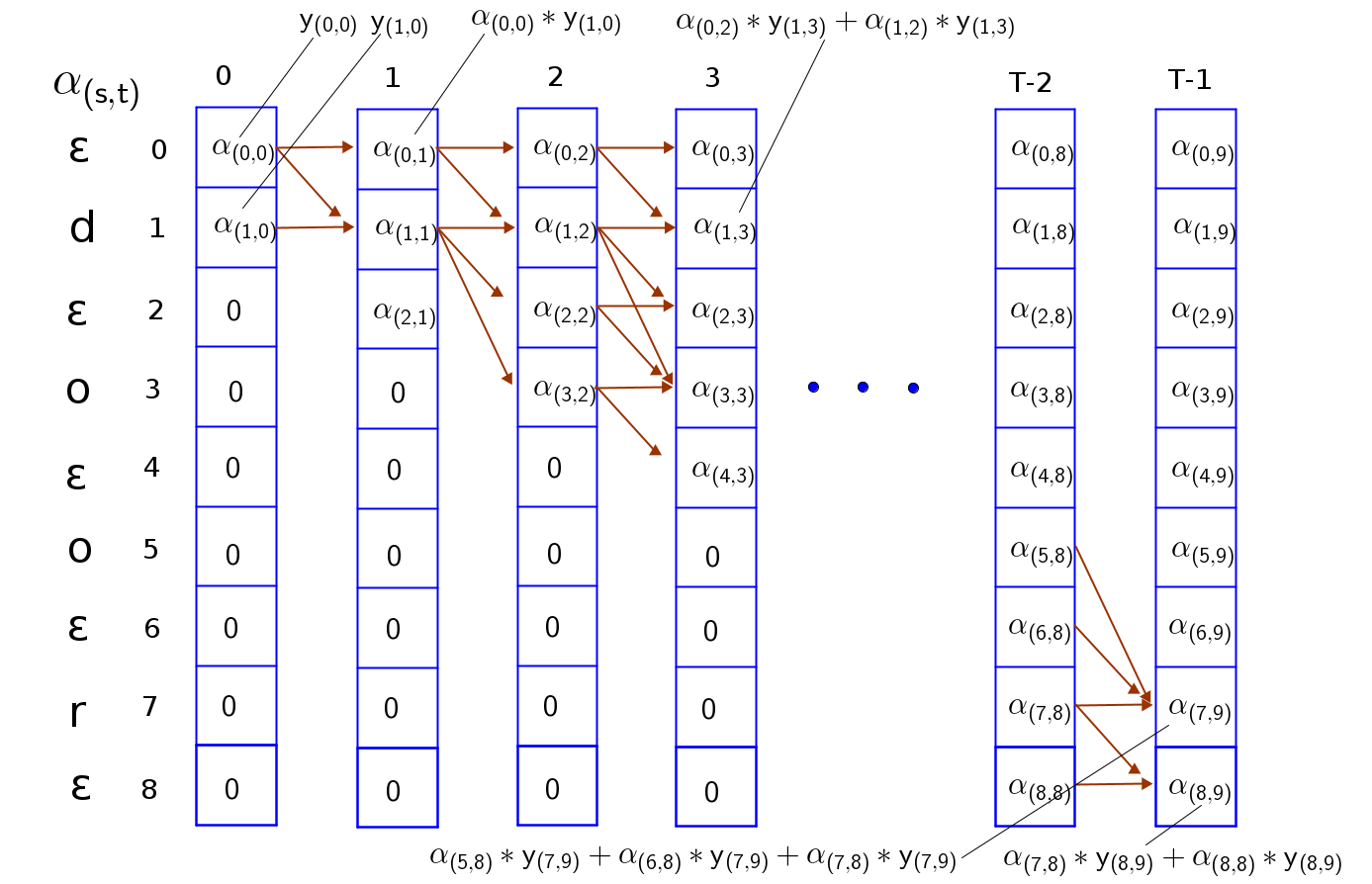
CTC Forward Algorithm: Alpha Pass Visualization — A visualization of the forward algorithm's progression. The arrows show valid transitions between states in the expanded sequence Z (here, for 'door'). The value at each node is computed based on the values from valid preceding nodes. Source: Sewade Ogun.

3.2. The Forward Pass ( $α$ )

We define the forward variable, $α_{s, t}$ , as the total probability of all paths that end at token $Z_{s}$ at time step $t$ .

Initialization ( $t = 1$ ):
At the first time step, a valid path can only be in one of two states: the initial blank ( $Z_{1} = ϵ$ ) or the first true character ( $Z_{2}$ ).

$α_{1, 1} = p_{1} (Z_{1} ∣ X)$ (Probability of blank at t=1)
$α_{2, 1} = p_{1} (Z_{2} ∣ X)$ (Probability of the first character at t=1)
$α_{s, 1} = 0$ for all $s > 2$ .

Recursion ( $t > 1$ ):
For any subsequent time step $t$ , the value of $α_{s, t}$ is calculated based on the $α$ values at the previous time step, $t - 1$ . We have two main cases for the transitions, which depend on the character $Z_{s}$ :

Case 1: No skip allowed. This happens if $Z_{s}$ is a blank token or if it's a character that's the same as the one two positions before it ( $Z_{s} = Z_{s - 2}$ ). This rule enforces that a blank must separate repeated characters. A path reaching $(s, t)$ could only have come from $(s, t - 1)$ (staying at the same character) or $(s - 1, t - 1)$ (moving from the previous character).
$α_{s, t} = (α_{s, t - 1} + α_{s - 1, t - 1}) \cdot p_{t} (Z_{s} ∣ X)$
Case 2: Skip allowed. If $Z_{s}$ is a unique character (i.e., $Z_{s} \neq = Z_{s - 2}$ ), a path is allowed to "skip" the preceding blank token ( $Z_{s - 1}$ ). This means a path reaching $(s, t)$ could have come from three places: $(s, t - 1)$ , $(s - 1, t - 1)$ , or $(s - 2, t - 1)$ .
$α_{s, t} = (α_{s, t - 1} + α_{s - 1, t - 1} + α_{s - 2, t - 1}) \cdot p_{t} (Z_{s} ∣ X)$

By applying this recursion from $t = 1$ to $T$ , we populate the entire trellis.

Final Probability:
A valid complete path must end at either the final character of $Z$ (at index $S$ ) or the final blank (at index $S - 1$ ). Therefore, the total probability $p (Y ∣ X)$ is the sum of the forward variables for these two states at the final time step $T$ :

p (Y ∣ X) = α_{S, T} + α_{S - 1, T}

And the CTC loss is simply $- lo g (p (Y ∣ X))$ .

3.3. The Backward Pass ( $β$ ) and Gradients

To train the network, we need to compute the gradient of the loss with respect to each network output $p_{t} (k ∣ X)$ . This requires the backward pass.

We define a backward variable, $β_{s, t}$ , as the total probability of all paths from time step $t$ at character $Z_{s}$ to the end of the sequence. The recursion for $β$ is symmetric to that of $α$ , but proceeds backward from time $T - 1$ to 1.

The product $α_{s, t} β_{s, t}$ gives the total probability of all valid paths for $Y$ that pass through state $s$ at time $t$ . Summing this product over all states $s$ at a given time $t$ gives the total probability $p (Y ∣ X)$ . This quantity is the key to calculating the gradient for backpropagation. While the full gradient derivation is quite involved, the crucial insight is that the forward and backward variables provide all the necessary components.

Breaking down the CTC Loss

For a clear, step-by-step derivation of both the forward and backward recursions, this blog post is an excellent resource.

Read the sections "Forward-Backward Algorithm" and "CTC Loss calculation for each timestep". This provides the explicit formulas for both alpha and beta and shows how they are combined.

4. A Practical Walkthrough with Code

The mathematical derivation can be abstract. Let's ground it by walking through a code implementation. Your experience with PyTorch and general software development will make this particularly insightful.

Connectionist Temporal Classification (CTC) From Scratch

The video "Connectionist Temporal Classification (CTC) From Scratch" by Priyam Mazumdar provides a fantastic, line-by-line implementation of the CTC forward pass in PyTorch. It perfectly bridges the gap between the math we've discussed and the tensor manipulations required to make it work.

This video is quite dense, so we will treat it as a guided code review. I'll break it down into segments corresponding to our derivation steps. I recommend having the video open and pausing as you go through my notes below. Dynamic Programming Concept & Rules (09:50 - 18:08): The video first motivates dynamic programming and explains the valid transition rules (Case 1 vs. Case 2 from our derivation). This provides a great visual intuition. Preparing the Tensors (18:08 - 21:31 & 37:09 - 43:34): This part covers two key pre-computation steps: Interleaving blanks: Modifying the target sequence to create Z. Creating the diff_labels mask: This boolean mask efficiently determines where a two-step transition (skip) is allowed (our Case 2). This is a clever implementation detail for handling the different recursion rules. Initializing the log_alpha Matrix (51:34 - 01:02:35): Here, the algorithm initializes the DP table. Notice two crucial details: Everything is done in log space (log_alpha) to prevent numerical underflow. Instead of multiplying probabilities, we add log-probabilities. The initial values for t=0 are set for the first blank and the first real character, just as in our initialization step. The matrix is padded with dummy values to simplify indexing. The Main DP Loop (01:02:35 - 01:15:00): This is the core of the forward pass. The code iterates through each time step t and calculates the log_alpha values for that step. Observe how it calculates the probabilities from the three possible previous states (stay, one-step, and two-step) and combines them using log-sum-exp. The two-step transition is masked by diff_labels. Final Loss Calculation (01:15:00 - 01:25:25): After the loop, the final probability is the log-sum-exp of the log-alphas of the last two valid states at the final time step. The video also shows verification against PyTorch's native CTCLoss, confirming the implementation's correctness.

This walkthrough demonstrates how the abstract recursion formulas are translated into efficient tensor operations, a skill that is central to practical AI/ML research and development. The use of log-space computations and masking are standard practice for robust numerical algorithms.

Conclusion

In this lesson, we have thoroughly dissected the Connectionist Temporal Classification loss function. You have moved from a high-level conceptual understanding to a detailed mathematical and practical one.

Key Takeaways:

The CTC objective is to maximize the log-likelihood of the correct transcript by summing the probabilities of all valid alignments that collapse to it.
A naive summation is computationally intractable due to the exponential number of paths.
The forward-backward algorithm, a dynamic programming technique, solves this efficiently by computing the sum in polynomial time.
The forward variable $α_{s, t}$ represents the total probability of all valid paths ending at state $s$ at time $t$ .
The backward variable $β_{s, t}$ represents the total probability of all valid paths starting from state $s$ at time $t$ .
The CTC loss is $- lo g (α_{S, T} + α_{S - 1, T})$ , calculated by the forward pass. The backward pass is required to efficiently compute gradients for training.
Practical implementations must operate in log-space to maintain numerical stability, using the log-sum-exp trick for addition.

Preview of the Next Lesson:

Now that we understand how to train a model using the CTC loss, the next logical step is to understand how to use that trained model for inference. In the next lesson, we will focus on decoding: given the probability matrix from a trained CTC model, how do we find the most likely output sequence? We will explore both simple greedy decoding and the more sophisticated beam-search algorithm.