CTC Decoding: Greedy & Beam Search

Hello!

In our previous lesson, we delved into the mathematics of the Connectionist Temporal Classification (CTC) loss function. You learned how the forward-backward algorithm efficiently computes the total probability of a target transcript by summing over all valid alignments, making it possible to train ASR models without needing a frame-by-frame alignment.

Now that we have a model trained with the CTC loss, we need to use it for inference. This lesson tackles the next logical step: decoding. Given the probability matrix output by our acoustic model, how do we extract the most likely text sequence? This lesson directly addresses the learning outcome: Implement greedy and beam-search decoding algorithms for a CTC output probability matrix.

We will start with the simplest approach, greedy search, and understand its limitations. Then, we'll dive into the more sophisticated and effective beam search algorithm, focusing on the specific adaptations required for CTC.

1. The Decoding Problem

After training, our acoustic model takes an audio input and outputs a probability matrix of size $T\times C$, where $T$ is the number of time steps (e.g., audio frames) and $C$ is the number of characters in our vocabulary (including the blank token, $ϵ$).

The goal of decoding is to find the most probable sequence $Y^{\ast }$ given the model's output probabilities, which we get from the input audio $X$. Formally, we want to solve:

Remember from the last lesson that $p(Y|X)$ is the sum of probabilities of all paths that collapse to $Y$. Finding the true maximum is a hard problem. We'll explore two algorithms that approximate this solution.

2. Greedy Search (Best Path Decoding)

The most straightforward approach is greedy search, also known as best path decoding. The algorithm is simple and intuitive:

1. For each time step $t$ from 1 to $T$, find the character with the highest probability.
2. Concatenate these characters to form the "best path," ${\pi }^{\ast }$.
3. Collapse this path using the CTC rules:
   a. Merge consecutive repeated characters.
   b. Remove all blank tokens.

Let's implement this. Given a log_probs matrix of shape (T, C), we can write a simple function.

import numpy as np

def greedy_decode(log_probs, vocab):
    """
    Performs greedy (best path) decoding.

    Args:
        log_probs (np.ndarray): A (T, C) matrix of log-probabilities.
        vocab (list): A list of characters corresponding to the indices.
                      (Assumes blank is at index 0).

    Returns:
        str: The decoded text.
    """



    # Find the character with the max probability at each time step
    best_path_indices = np.argmax(log_probs, axis=1)




    # Collapse repeats
    collapsed_path = []
    for i, idx in enumerate(best_path_indices):
        if i > 0 and idx == best_path_indices[i-1]:
            continue
        collapsed_path.append(idx)




    # Remove blanks
    decoded_indices = [idx for idx in collapsed_path if idx != 0]




    # Convert indices to characters
    return "".join([vocab[idx] for idx in decoded_indices])




# --- Example Usage ---
# vocab = ['-', 'a', 'b', 'c'] # - is blank
# T=5, C=4
# log_probs = np.array([
#     [-1.0, -2.3, -2.3, -2.3], # t0: blank
#     [-3.0, -1.2, -3.0, -3.0], # t1: 'a'
#     [-4.0, -1.1, -4.0, -4.0], # t2: 'a'
#     [-0.5, -3.0, -3.0, -3.0], # t3: blank
#     [-5.0, -5.0, -1.5, -5.0], # t4: 'b'
# ])


```grasp
{
  "type": "exercise",
  "id": "05439f76-6aab-4e11-bdad-4b87e93401e9"
}

best_path_indices would be [0, 1, 1, 0, 2] -> ['-', 'a', 'a', '-', 'b']

collapsed_path would be [0, 1, 0, 2] -> ['-', 'a', '-', 'b']

decoded_indices would be [1, 2] -> ['a', 'b']

result = "ab"

**Limitations of Greedy Search**

While fast and simple, greedy search is often suboptimal. It finds the single most likely path, $\pi^*$, but the probability of this single path, $p(\pi^*|X)$, is not the same as the total probability of a sequence, $p(Y|X) = \sum_{\pi \in \mathcal{B}^{-1}(Y)} p(\pi | X)$. A different, less probable path might collapse to a sequence that has a higher overall probability when summed with other valid paths.

```grasp
{
  "type": "reading",
  "title": "ASR Beam Search Implementation",
  "id": "[LINK](https://www.arunbaby.com/speech-tech/0023-asr-beam-search-implementation/)",
  "url": "https://www.arunbaby.com/speech-tech/0023-asr-beam-search-implementation/",
  "relevant_section_indices": [
    1
  ],
  "par_intro": "The article \"ASR Beam Search Implementation\" by Arun Baby provides a clear example of why this local, greedy approach can fail.",
  "par_directions": "Please read the short section titled \"Why Greedy Fails in Speech\". It perfectly illustrates how a locally optimal choice can lead to a globally suboptimal result.",
  "estimated_time": "3 minutes"
}

To find a better approximation of the true most likely sequence, we need a search algorithm that considers multiple hypotheses simultaneously.

3. Beam Search Decoding

Beam search is a heuristic search algorithm that improves upon greedy search by keeping a fixed number of the most promising candidate sequences, known as the "beam," at each time step.

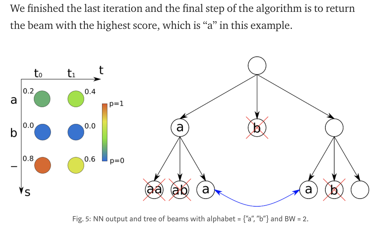
For standard sequence-to-sequence models, beam search is relatively straightforward. For CTC, it's more complex due to the blank token and the collapsing mechanism. The key challenge is that different paths can merge into the same output prefix. For example, both h-e and he collapse to he.

To handle this, a CTC beam search algorithm must track two separate probabilities for each prefix in the beam:

1. p_b: The probability of the prefix ending with a blank token.
2. p_nb: The probability of the prefix ending with a non-blank token.

Why is this distinction crucial? Consider the prefix "hel".

• If the next character is "l", and we came from a path ending in a non-blank (e.g., "hel"), the result is still "hel" (l + l merge).
• If the next character is "l", but we came from a path ending in a blank (e.g., "hel-"), the result becomes "hell" (l + $ϵ$ + l do not merge).

The algorithm proceeds as follows:

1. Initialization: Start with an empty prefix "" in the beam. Its p_b is 1 (or 0 in log space) and p_nb is 0 (-inf in log space).
2. Iteration: For each time step $t$:
   a. Create a next_beam.
   b. For each prefix in the current beam:
   i. Extend with blank: The prefix text doesn't change. Calculate its new p_b in the next_beam.
   ii. Extend with non-blanks: For each character c in the vocabulary:
   - Calculate the new prefix and its corresponding p_nb. This is where the p_b vs. p_nb logic is applied to handle merges correctly.
   c. Pruning: Sort all prefixes in next_beam by their total probability (p_b + p_nb) and keep only the top beam_width candidates.
   d. Replace the current beam with the pruned next_beam.
3. Finalization: After the last time step, the prefix with the highest total probability in the final beam is the result.

4. Implementing CTC Beam Search

Now, let's translate this algorithm into code. Given your background, walking through a Python implementation will solidify your understanding. We'll follow the logic from the article you just read, using a dictionary to store the beam and working in the log-probability space to maintain numerical stability.

We will use np.logaddexp which computes $\log (e^x+e^y)$. This is the equivalent of adding probabilities when you are working with log-probabilities.

import numpy as np
from collections import defaultdict

def ctc_beam_search_decoder(log_probs, vocab, beam_width=10):
    """
    Performs CTC beam search decoding.

    Args:
        log_probs (np.ndarray): (T, C) matrix of log-probabilities.
        vocab (list): Character vocabulary.
        beam_width (int): The number of hypotheses to keep in the beam.

    Returns:
        str: The best decoded string.
    """
    T, C = log_probs.shape
    



    # beam: maps prefix (tuple) -> (log_p_blank, log_p_non_blank)
    beam = defaultdict(lambda: (np.log(0), np.log(0)))
    



    # Initialize with empty prefix
    beam[()] = (np.log(1), np.log(0)) # (p_b=1, p_nb=0)

    for t in range(T):
        next_beam = defaultdict(lambda: (np.log(0), np.log(0)))
        



        # Sort prefixes by their total probability
        # We use logaddexp to sum probabilities in the log domain
        sorted_prefixes = sorted(
            beam.items(),
            key=lambda x: np.logaddexp(x[1][0], x[1][1]),
            reverse=True
        )[:beam_width]

        for prefix, (log_p_b, log_p_nb) in sorted_prefixes:



            # 1. Extend with BLANK
            pr_blank = log_probs[t, 0]



            # New blank score comes from total previous score
            # A- -> A-- (prefix doesn't change)
            # A  -> A-  (prefix doesn't change)
            n_log_p_b, n_log_p_nb = next_beam[prefix]
            total_prev_log_p = np.logaddexp(log_p_b, log_p_nb)
            next_beam[prefix] = (np.logaddexp(n_log_p_b, pr_blank + total_prev_log_p), n_log_p_nb)




            # 2. Extend with NON-BLANK characters
            for c_idx in range(1, C):
                pr_char = log_probs[t, c_idx]
                char = vocab[c_idx]
                



                # Case A: New character is a repeat of the last char in prefix
                if prefix and prefix[-1] == char:

```grasp
{
  "type": "exercise",
  "id": "6adfc434-9cdf-4be3-b398-23985437f5f8"
}

                # A -> A + A = A (merge). Comes from NON-BLANK path.
                n_log_p_b, n_log_p_nb = next_beam[prefix]
                next_beam[prefix] = (n_log_p_b, np.logaddexp(n_log_p_nb, pr_char + log_p_nb))
                



                # A- -> A- + A = AA (no merge). Comes from BLANK path.
                new_prefix = prefix + (char,)
                n_log_p_b, n_log_p_nb = next_beam[new_prefix]
                next_beam[new_prefix] = (n_log_p_b, np.logaddexp(n_log_p_nb, pr_char + log_p_b))
            



            # Case B: New character is different
            else:
                new_prefix = prefix + (char,)
                n_log_p_b, n_log_p_nb = next_beam[new_prefix]
                total_prev_log_p = np.logaddexp(log_p_b, log_p_nb)
                next_beam[new_prefix] = (n_log_p_b, np.logaddexp(n_log_p_nb, pr_char + total_prev_log_p))




    # Update the beam for the next time step
    beam = next_beam




# Final selection
best_prefix_tuple = max(beam.items(), key=lambda x: np.logaddexp(x[1][0], x[1][1]))[0]
return "".join(best_prefix_tuple)

This implementation directly mirrors the logic we discussed. It iterates through time, expands hypotheses, correctly applies the CTC merging rules based on the blank/non-blank state, and prunes the search space.

For reference, several open-source libraries provide optimized implementations of these algorithms. The `CTCDecoder` repository is a good example of a standalone Python package for this purpose.

```grasp
{
  "type": "reading",
  "title": "CTC Decoding Algorithms",
  "id": "[LINK](https://github.com/githubharald/CTCDecoder)",
  "url": "https://github.com/githubharald/CTCDecoder",
  "relevant_section_indices": [
    1,
    2
  ],
  "par_intro": "The following GitHub repository provides packaged implementations of the decoders we've discussed.",
  "par_directions": "Briefly look at the \"Usage\" and \"List of provided decoders\" sections. This shows how you would use a pre-built library for `best_path` and `beam_search` decoding, which is what you would typically do in a practical project.",
  "estimated_time": "2 minutes"
}

Conclusion

In this lesson, we transitioned from training a CTC model to performing inference with it. You learned how to transform the raw probability matrix from an acoustic model into human-readable text.

Key Takeaways:

• Decoding is the process of finding the most likely output sequence from a model's probability distribution.
• Greedy Search (Best Path Decoding) is a simple, fast algorithm that picks the most likely character at each time step. It's often suboptimal because the most likely path doesn't always correspond to the most likely overall sequence.
• Beam Search Decoding is a more effective heuristic that maintains a beam_width of promising hypotheses at each step, preventing premature decisions.
• CTC Beam Search is more complex than standard beam search. It requires tracking two probabilities for each hypothesis—one for paths ending in a blank (p_b) and one for paths ending in a non-blank (p_nb)—to correctly handle CTC's character-merging rules.

Preview of the Next Lesson:

Our beam search implementation uses only the acoustic model's probabilities. However, we know that some sequences of characters (and words) are much more likely than others in a given language (e.g., "recognize speech" is more likely than "wreck a nice beach"). In the next lesson, we will explore how to integrate a Language Model (LM) into the beam search process to further improve decoding accuracy. This process, known as shallow fusion, combines the acoustic score with a language model score to find outputs that are both acoustically and linguistically plausible.