Speech Recognition: Sequence-to-Sequence and Alignment Challenges

Hello! Welcome to the sixth module of our course. In the previous module, we explored the foundations of deep generative modeling, comparing the strengths and weaknesses of VAEs, GANs, and Flow-based models. We're now going to pivot from unsupervised generation to a core supervised task in audio AI: Automatic Speech Recognition (ASR).

Your experience with models like Whisper has given you a practical sense of what ASR can do. Our goal now is to peel back the layers and understand the fundamental problem these models are designed to solve.

Today's lesson focuses on the learning outcome: Formulate speech recognition as a sequence-to-sequence problem and explain the alignment challenge. We will define the ASR task formally, understand why it's so difficult, and introduce the two main conceptual frameworks—Connectionist Temporal Classification (CTC) and attention mechanisms—that form the basis of modern solutions.

1. From Complex Pipelines to End-to-End Systems

Modern ASR systems that map raw audio directly to text are often called "end-to-end" models. To appreciate why this is a significant development, it's helpful to first understand the classical approach.

As the video explained, traditional ASR systems are modular pipelines, typically consisting of:

1. Acoustic Model (AM): Maps short audio frames (features like MFCCs) to probabilities of phonetic units (phonemes). This is where a neural network was often first introduced to replace older methods like Gaussian Mixture Models (GMMs).
2. Pronunciation Model (or Lexicon): A dictionary that maps sequences of phonemes to words. For example, it knows that the phoneme sequence /k/ /æ/ /t/ corresponds to the word "cat".
3. Language Model (LM): Assigns probabilities to sequences of words (e.g., "how are you" is more probable than "how are shoe"). This helps resolve ambiguity and correct errors from the acoustic model.

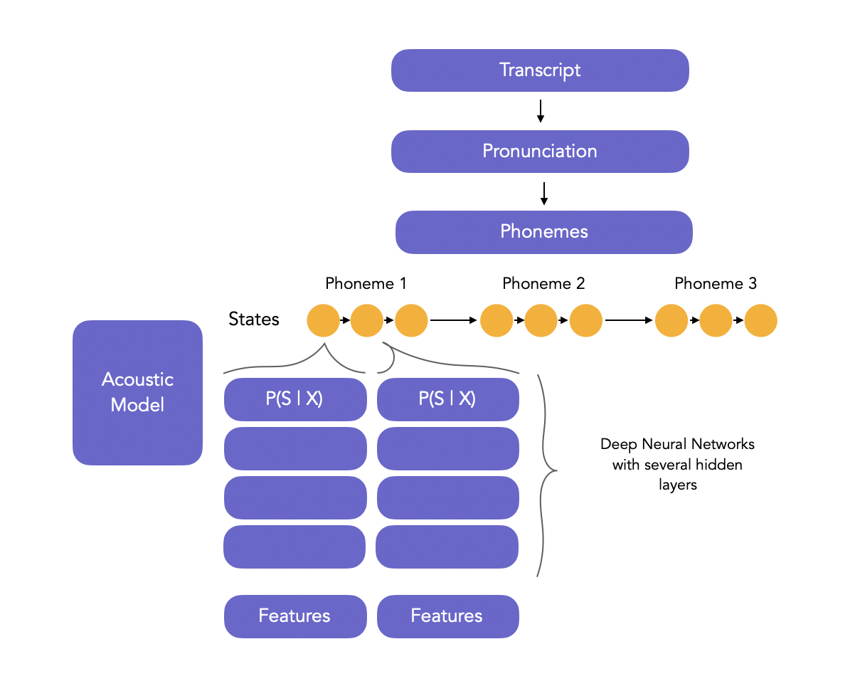
The key takeaway is that this traditional approach required hand-engineered components, linguistic expertise (for phonemes), and careful, separate tuning of each part. The "neural network invasion" replaced these parts one by one, which naturally led to the next question: Can we replace the entire pipeline with a single, unified neural network?

This is the core idea of end-to-end ASR: learning a single function that maps a sequence of audio inputs, $X$, directly to a sequence of text outputs, $Y$. We want to model the conditional probability $P(Y|X)$.

2. ASR as a Sequence-to-Sequence (Seq2Seq) Problem

This "sequence of inputs to sequence of outputs" formulation is a general machine learning paradigm known as a sequence-to-sequence (Seq2Seq) problem. It's not unique to speech; machine translation ("Hello, how are you?" → "¿Hola, cómo estás?") is the classic example.

Let's watch a brief, clear explanation of Seq2Seq models.

As you just saw, the defining characteristic of a Seq2Seq problem is that the model must handle variable-length inputs and outputs, and the lengths don't have to match. This perfectly describes ASR:

• Input Sequence $X$: A sequence of feature vectors, $X=[x_1,x_2,\dots ,x_T]$, where each $x_t$ is a frame of audio features (e.g., a slice of a mel-spectrogram). The length $T$ can be thousands of frames.
• Output Sequence $Y$: A sequence of tokens, $Y=[y_1,y_2,\dots ,y_U]$, where each $y_u$ is a character or a word. The length $U$ is typically much smaller than $T$.

The standard architecture for solving Seq2Seq problems is the Encoder-Decoder model.

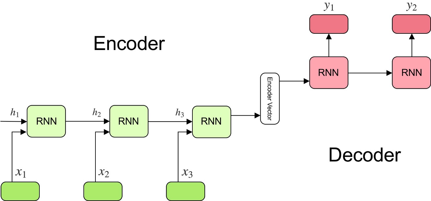
The architecture works as follows:

1. Encoder: A neural network (often a Recurrent Neural Network like an LSTM, or more recently, a Transformer) processes the entire input sequence $X$ and compresses its information into a fixed-size representation called a context vector. This vector is expected to be a meaningful summary of the entire audio input.
2. Decoder: Another neural network takes the context vector from the encoder as its initial state. It then generates the output sequence $Y$ one token at a time, with each generated token influencing the next.

This architecture elegantly decouples the input and output, allowing their lengths to be different. However, for ASR, there's a deeper, more fundamental challenge that this simple picture doesn't fully capture.

3. The Alignment Challenge

The core difficulty in ASR is that we don't know the alignment between the input audio frames and the output text characters. When you have a 10-second audio clip and a 50-character transcript, which specific milliseconds of audio correspond to the first character? Which correspond to the second? The answer is not obvious and is the central problem that ASR models must solve.

Let's read a concise and clear description of this problem.

The article you just read, along with this excellent summary from another resource, highlights the key facets of the alignment challenge:

To summarize, the alignment is difficult because:

• Length Mismatch: The input sequence $X$ (audio frames) is much longer than the output sequence $Y$ (characters). A single spoken character can span multiple audio frames.
• No Obvious Boundaries: Speech is a continuous signal. There are no clear markers in the waveform that say "character 'c' ends here, character 'a' begins here."
• Rate Variation: People speak at different speeds. The duration of a phoneme for a given character can vary significantly.
• Repeated Characters vs. Elongation: In the word "hello", the audio for the 'l' sound is elongated. How does a model know to output "ll" instead of just a single "l"?
• Pauses and Non-speech: Audio contains silence, breaths, and filler words ("um", "uh"). The model must learn to ignore or filter these out, producing no corresponding output characters.

Manually aligning every character in a large dataset is prohibitively expensive. Therefore, the most successful ASR models are those that can learn this alignment automatically.

4. Two Primary Approaches to Automatic Alignment

Modern end-to-end ASR models generally use one of two main strategies to solve the alignment problem.

Approach 1: Connectionist Temporal Classification (CTC)

CTC provides an ingenious way to train an ASR model without an explicit alignment.

The core ideas behind CTC are:

1. Frame-wise Prediction: The model (typically an RNN or Transformer) predicts a character probability distribution for every single input frame. This results in a very long sequence of predictions, equal in length to the input audio frames ($T$).
2. The Blank Token (ϵ): The output vocabulary is augmented with a special blank token. This token represents "not a character" and can be emitted for frames corresponding to pauses or the transitions between characters.
3. The Collapse Function: A simple set of rules defines how to map the long prediction sequence to the final output:
   • First, merge all consecutive repeated characters (e.g., h, h, e, l, l, l, o → h, e, l, o).
   • Second, remove all blank tokens (e.g., ϵ, c, ϵ, a, a, t, ϵ → c, a, a, t → c, a, t).

The blank token is crucial for handling repeated characters. An alignment for "hello" must have a blank between the two 'l's (e.g., h, e, l, ϵ, l, o) to prevent them from being collapsed into a single 'l'.

CTC works by calculating a loss function that sums the probabilities of all possible valid alignments that could collapse to the correct transcript. This allows the model to learn without ever needing to commit to a single, hard alignment.

Approach 2: Attention-Based Encoder-Decoder

The second approach tackles alignment in a more direct, but still learned, fashion using an attention mechanism.

In an attention-based model:

1. The Encoder (the "Listen" part) processes the entire audio sequence to produce a set of rich hidden states, one for each input frame.
2. The Decoder (the "Spell" part) generates the output transcript one character at a time.
3. At each step, before producing the next character, the decoder uses an Attention Mechanism (the "Attend" part). It compares its current internal state to all of the encoder's hidden states to compute an "attention vector". This vector assigns high weights to the audio frames that are most relevant for predicting the next character.
4. The decoder then uses a weighted average of the encoder states (weighted by the attention vector) to inform its prediction.

In essence, the model learns to align by itself. As it generates the transcript, the "spotlight" of its attention moves across the audio, focusing on the relevant parts for each character it writes.

Conclusion

In this lesson, we have formally defined the problem of automatic speech recognition and framed it within the powerful sequence-to-sequence paradigm.

Key Takeaways:

• ASR can be formulated as a sequence-to-sequence problem, mapping a long sequence of audio features ($X$) to a much shorter sequence of text tokens ($Y$).
• The fundamental difficulty in ASR is the alignment challenge: the mapping between the continuous, variable-rate audio signal and the discrete text transcript is unknown.
• Manually creating this alignment is impractical, so modern ASR models must learn it automatically.
• Two dominant paradigms for automatic alignment are:
  • Connectionist Temporal Classification (CTC): Makes a prediction per audio frame and uses a blank token and a collapsing function to map the long prediction sequence to the short output sequence, marginalizing over all possible alignments.
  • Attention Mechanisms: An encoder-decoder model where the decoder learns to focus on the most relevant parts of the input audio at each step of generating the output.

Preview of the Next Lesson:

We have introduced the high-level concept of CTC as a solution to the alignment problem. In our next lesson, we will get into the details. We will derive the Connectionist Temporal Classification (CTC) loss function and understand the forward-backward algorithm that makes its computation tractable. This will give you a deep mathematical understanding of one of the most important algorithms in modern ASR.