Activation Memory Calculation

Introduction

Welcome back! In our previous lesson, we established the first pillar of LLM memory calculation: the static VRAM required to store a model's weights. You learned that Model Memory = Num Parameters × Bytes per Parameter, which explains why a 70B parameter model in half-precision (fp16) demands a baseline of 140 GB VRAM.

However, loading the weights is just the beginning. The moment we perform a forward pass—that is, ask the model to generate text—a new, dynamic component of memory usage appears: activations. These are the intermediate tensors created as data flows through the model's layers. While the model weights are static, activation memory grows and shrinks with every computation.

This lesson directly addresses the learning outcome: Calculate the activation memory consumed during a forward pass for a given batch size and sequence length. Mastering this will give you the second major piece of the VRAM puzzle, bringing you closer to fully explaining why a model's memory footprint can be much larger than its weights alone.

What Are Activations and Why Do They Consume VRAM?

During a forward pass, the output of one operation becomes the input for the next. For example, the output of an attention block is fed into a feed-forward network. These intermediate results are called "activations."

• During training, frameworks like PyTorch must cache all activations from the forward pass. This is because they are required by the autograd engine to compute gradients during the backward pass. This leads to very high memory consumption.

• During inference, we don't perform a backward pass, so there's no need to cache activations from all layers simultaneously. As soon as a layer's computation is finished, the memory holding its input activation can theoretically be reused. However, within the computation of a single transformer layer, multiple intermediate tensors are created and must exist in memory at the same time. The VRAM required to hold these transient tensors at the moment of highest demand is the peak activation memory.

Our focus for LLM serving is on this peak inference memory, which is typically dominated by the calculations within a single, complex transformer layer.

Anatomy of Activation Memory in a Transformer Layer

To calculate the activation memory, we must look inside a standard decoder-only transformer layer. It primarily consists of two sub-modules:

1. Multi-Head Attention (MHA)
2. Feed-Forward Network (FFN)

Each of these modules, along with Layer Normalization, creates temporary tensors during its computation.

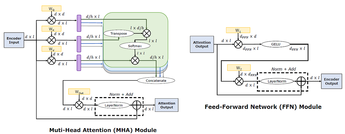
The peak activation memory for the entire model during inference is the maximum memory needed to execute any single one of these layers. Since all transformer layers are typically identical, we just need to calculate it for one.

Calculating Peak Activation Memory for Inference

To calculate the memory, we first need to define our key hyperparameters:

• s: sequence length (number of tokens being processed)
• b: batch size (number of sequences processed in parallel)
• h: hidden dimension size (d_model)
• i: intermediate dimension of the FFN (often 4 * h)
• a: number of attention heads

We will assume all activations are stored in a 16-bit format (like fp16 or bf16), meaning each numerical value requires 2 bytes.

The following blog post provides a detailed breakdown of these calculations specifically for the inference case.

Based on the article and common transformer architectures, we can approximate the peak activation memory for a single layer as the sum of the memory needed for its constituent parts.

1. Attention Block Memory

This memory is used for storing the query (Q), key (K), value (V) matrices, and the results of their intermediate multiplications. A good approximation, assuming an optimized implementation like FlashAttention (which avoids materializing the full s x s attention matrix), is:

$${\text{Memory}}_{\text{Attention}}\approx 10\times s\times b\times h\times (\text{bytes per element})$$

With fp16 (2 bytes), this becomes:

$${\text{Memory}}_{\text{Attention}}\approx 20\times s\times b\times h\text{ bytes}$$

2. Feed-Forward Network (FFN) Memory

Modern LLMs like Llama use a gated FFN (or SwiGLU), which involves parallel linear projections (gate_proj, up_proj) followed by a final down_proj. The peak memory occurs when we need to store the inputs to these projections simultaneously.

The formula from the article, 4 * s * b * (i + h), represents this. It accounts for storing the original input x (size s*b*h) for two projections and the intermediate results (size s*b*i) for the activation function and the final projection.

$${\text{Memory}}_{\text{FFN}}\approx 4\times s\times b\times (i+h)\times (\text{bytes per element})$$

With fp16 (2 bytes) and a standard FFN where i ≈ 4h:

$${\text{Memory}}_{\text{FFN}}\approx 8\times s\times b\times (4h+h)=8\times s\times b\times 5h=40\times s\times b\times h\text{ bytes}$$

3. Layer Normalization Memory

A transformer layer typically has two LayerNorm operations. Each needs to hold a copy of its input tensor.

$${\text{Memory}}_{\text{LayerNorm}}=2\times (s\times b\times h)\times (\text{bytes per element})$$

With fp16 (2 bytes):

$${\text{Memory}}_{\text{LayerNorm}}=4\times s\times b\times h\text{ bytes}$$

Total Peak Activation Memory per Layer

Combining these components gives us the total peak activation memory for one layer's forward pass:

$${\text{Memory}}_{\text{Activation\_Peak}}={\text{Memory}}_{\text{Attention}}+{\text{Memory}}_{\text{FFN}}+{\text{Memory}}_{\text{LayerNorm}}$$ $${\text{Memory}}_{\text{Activation\_Peak}}\approx (20+40+4)\times s\times b\times h=\text{64}\times s\times b\times h\text{ bytes}$$

This is our working formula. It demonstrates that activation memory scales linearly with batch size, sequence length, and hidden dimension.

Practical Example: Llama-2 7B

Let's apply this to a real model. For Llama-2 7B:

• h (hidden dimension) = 4096
• i (intermediate dimension) = 11008 (approx. 2.7 * h)
• Let's assume s = 1024 and b = 1.

Let's use the more precise formulas for a Llama-style model:

• Memory_Attention = 20 * 1024 * 1 * 4096 = 83.9 MB
• Memory_FFN = 8 * 1024 * 1 * (11008 + 4096) = 123.7 MB
• Memory_LayerNorm = 4 * 1024 * 1 * 4096 = 16.8 MB

Total Peak Activation Memory:
83.9 + 123.7 + 16.8 = 224.4 MB

This is the transient memory required for a single forward pass through one layer. While this seems small, remember this is for a batch size of 1. If you serve a batch of 32 requests (b=32), this peak memory jumps to 224.4 MB * 32 = 7.2 GB, which is a substantial portion of a GPU's VRAM.

Self-Check Exercise

Now it's your turn. Calculate the approximate peak activation memory for a forward pass with the following parameters, using our simplified formula (64 * s * b * h):

• Model Type: A 3B parameter model
• h (hidden dimension) = 3072
• s (sequence length) = 2048
• b (batch size) = 8
• Precision: fp16 (activations are 2 bytes each)

...

Answer:

First, let's calculate the total number of elements:
s * b * h = 2048 * 8 * 3072 = 50,331,648

Now, apply our formula for bytes:
Memory = 64 * s * b * h = 64 * 50,331,648 = 3,221,225,472 bytes

Finally, convert bytes to gigabytes (dividing by 1024³):
3,221,225,472 / (1024**3) ≈ 3.0 GB

So, a batch of 8 sequences of length 2048 would consume approximately 3.0 GB of transient activation memory during the forward pass of each layer.

Conclusion

In this lesson, you've added the second major component to your VRAM calculation model. You can now estimate the dynamic memory consumed by activations during a forward pass.

Key Takeaways:

• Activation memory is dynamic and transient, required for the intermediate calculations within a transformer layer during a forward pass.
• For inference, we care about the peak activation memory for a single layer, as this memory is reused.
• Activation memory scales linearly with batch_size, sequence_length, and hidden_dim.
• The formula Memory_Activation ≈ 64 * s * b * h bytes provides a good rule-of-thumb for 16-bit precision, capturing the combined memory needs of the attention and FFN blocks.
• Even for moderate batch sizes, activation memory can become a significant consumer of VRAM, competing with the memory needed for model weights and the KV cache.

Preview of the Next Lesson:

We've covered the model weights (static) and the activations (transient). But there's a third, crucial piece of the memory puzzle, one that is responsible for the "out of memory" errors when generating long sequences: the KV Cache. In the next lesson, we will analyze the forward pass of a decoder block, mapping operations to their compute and memory costs, which will set the stage for a deep dive into calculating the KV cache size in the lesson that follows.