VRAM for Model Weights: Parameter Count & Data Type

Introduction

In our last lesson, we demystified the process of counting a transformer's parameters, culminating in a Python function and a powerful rule of thumb (L * 12 * d_model^2) to estimate a model's size. You can now look at a model's hyperparameters and determine how many millions or billions of parameters it contains.

This lesson takes the crucial next step. We will translate that abstract parameter count into a concrete, physical resource requirement: GPU VRAM. This directly addresses one of the core questions of this course: "Why is my 70B model using 120 GB of VRAM?"

Our goal is to master the learning outcome: Calculate the VRAM required to store model weights for a given parameter count and data type (fp32, fp16, bf16). This calculation forms the absolute baseline for any LLM memory analysis.

The Language of Precision: From Parameters to Bytes

The number of parameters alone doesn't tell us the memory footprint. The missing piece is the numerical precision used to store each parameter. Each parameter in a model is a floating-point number, and the amount of memory it occupies depends on its data type.

The most common data types in deep learning are:

• fp32 (single precision): The standard 32-bit floating-point format.
• fp16 (half precision): A 16-bit format that saves memory at the cost of reduced precision and range.
• bf16 (brain float): Another 16-bit format, developed by Google, which prioritizes a large dynamic range (like fp32) over precision.

The image below shows how the 32 or 16 bits are allocated for each type.

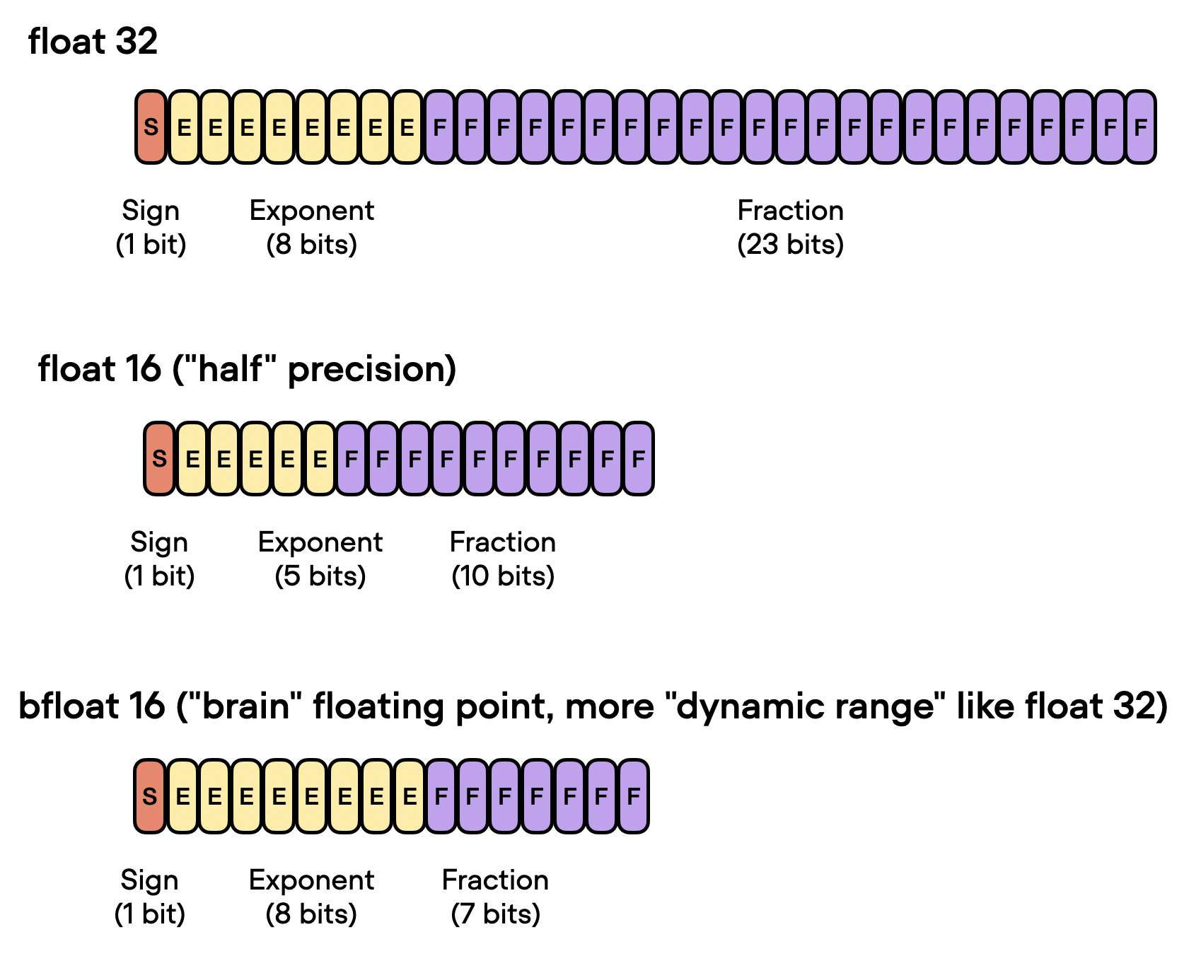
To fully grasp the implications of these differences, let's dive into their structure. Given your CS background, a bit-level understanding will provide a solid foundation for why these types behave differently, especially when we discuss quantization later.

The crucial takeaway for our VRAM calculation is the number of bytes each parameter occupies:

• fp32: 32 bits = 4 bytes
• fp16: 16 bits = 2 bytes
• bf16: 16 bits = 2 bytes

The Fundamental Formula for Model Weight Memory

With the bytes-per-parameter established, the calculation for storing the model weights becomes straightforward. You simply multiply the number of parameters by the bytes required for the chosen data type.

As the article states, the formula is:

$$\text{Model Memory (bytes)}=\text{Number of Parameters}\times \text{Bytes per Parameter}$$

To convert this to gigabytes (GB), you divide by $1024^3$. However, a common and useful convention in the field is to approximate 1 billion bytes as 1 GB. We will use this simpler convention for our estimates.

Calculation in Practice: The 70B Model Case

Let's apply this to answer one of the course's framing questions. A 70 billion parameter model is a standard large model size (e.g., Llama-2 70B).

Scenario 1: Using Full Precision (fp32)

• Parameters: 70,000,000,000
• Bytes per parameter: 4
• Calculation: 70B params * 4 bytes/param = 280B bytes
• VRAM Required: ~280 GB

Scenario 2: Using Half Precision (fp16 or bf16)

• Parameters: 70,000,000,000
• Bytes per parameter: 2
• Calculation: 70B params * 2 bytes/param = 140B bytes
• VRAM Required: ~140 GB

This simple calculation reveals a critical insight: even with half-precision, a 70B model's weights alone require 140 GB of VRAM. This is why a single NVIDIA A100 GPU with 80 GB of VRAM cannot load the model without further optimizations like quantization or model parallelism, which we will cover in future modules.

Overhead and Practical Estimation Tools

The VRAM needed for model weights is the non-negotiable baseline. However, it's not the only consumer of memory. During inference, other components also require VRAM:

• Activations: Intermediate results from calculations within the model layers.
• KV Cache: Stores attention states for previously processed tokens.
• Framework Overhead: Memory used by PyTorch, CUDA kernels, etc.

For a quick but more holistic estimate, a common practice is to add a small overhead margin (e.g., 20%) to the weight memory.

While we will deconstruct each overhead component (activations, KV cache) in subsequent lessons, this gives you a complete first-pass mental model for VRAM estimation. For this lesson, our focus remains on precisely calculating the weight component.

Self-Check Exercise

Let's test your understanding. Calculate the VRAM required to store the weights of a 13B parameter model (like Llama-2 13B) using the following data types. We'll also include INT8 as a preview for our upcoming lessons on quantization.

• fp32 (4 bytes)
• fp16 (2 bytes)
• INT8 (1 byte)

...

Answers:

• fp32: 13B * 4 bytes = 52 GB
• fp16: 13B * 2 bytes = 26 GB
• INT8: 13B * 1 byte = 13 GB

Notice how moving from fp16 to INT8 halves the memory requirement again. This is the power of quantization. For quick reference, the table below (from the Propelrc blog LINK) shows typical VRAM requirements for various model sizes, which aligns with our calculations.

Model Size	FP16 VRAM	INT8 VRAM	INT4 VRAM
3B parameters	6-8GB	3-4GB	1.5-2GB
7B parameters	14-16GB	7-8GB	3.5-4GB
13B parameters	26-30GB	13-15GB	6.5-7.5GB
70B parameters	140-150GB	70-75GB	35-38GB

Conclusion

In this lesson, you've connected the abstract concept of parameters to the physical reality of VRAM consumption. You can now perform the most fundamental calculation in LLM systems engineering.

Key Takeaways:

• VRAM for model weights is calculated as: Number of Parameters * Bytes per Parameter.
• The choice of data type is critical: fp32 uses 4 bytes, while fp16 and bf16 use 2 bytes, instantly halving the memory footprint.
• This weight memory is the static baseline. Total VRAM usage will be higher due to dynamic components like activations and the KV cache.
• Even for moderately sized models (13B+), fp16 precision is essential to fit on most single consumer or enterprise GPUs.

Preview of the Next Lesson:

We've now quantified the memory that is statically occupied by just loading the model. But what happens when we perform a forward pass? The moment we feed data into the model, a new, dynamic memory consumer appears: activations. In our next lesson, we will learn to calculate the activation memory consumed during a forward pass for a given batch size and sequence length, adding another critical piece to our VRAM puzzle.