Decoder Block: Compute & Memory Analysis

Introduction

Welcome back. In the previous lesson, we moved from calculating static model weight memory to understanding the dynamic memory consumed by activations. We established a high-level formula (Memory_Activation ≈ 64 * s * b * h) that approximates the peak transient VRAM needed for a forward pass. This formula is a useful rule of thumb, but to truly answer "Why is my model slow?", we need to go deeper than just memory size.

This lesson directly addresses the learning outcome: Analyze the forward pass of a decoder block, mapping operations to their respective compute (MatMul) and memory (data movement) costs. We will dissect the operations inside the Multi-Head Attention (MHA) and Feed-Forward Network (FFN) blocks, quantifying their costs in two fundamental units:

• Compute Cost: The number of floating-point operations (FLOPs).
• Memory Cost: The amount of data moved to and from the GPU's main memory (I/O).

By the end of this lesson, you will understand why different parts of the inference process have vastly different performance characteristics and why simply looking at FLOPs can be misleading.

Compute-Bound vs. Memory-Bound Operations

At its core, a GPU consists of processing units (like SMs) that perform calculations and high-bandwidth memory (HBM) that stores data. The performance of any operation is limited by one of these two factors.

• Compute-Bound: An operation is compute-bound if the time it takes is limited by the GPU's processing speed (TFLOPS). The GPU cores are fully utilized, working on calculations as fast as they can. Classic examples are large, dense matrix multiplications.
• Memory-Bound: An operation is memory-bound if its speed is limited by the rate at which data can be transferred from HBM to the processing units (memory bandwidth, in GB/s). The GPU cores spend much of their time waiting for data to arrive. Element-wise operations like ReLU or LayerNorm are classic examples.

To formalize this, we use a key metric: Arithmetic Intensity (AI).

$$\text{Arithmetic Intensity (AI)}=\frac{\text{Total FLOPs}}{\text{Total Bytes Transferred (I/O)}}$$

An operation with high AI performs many calculations for each byte of data it reads, making it likely to be compute-bound. An operation with low AI does few calculations per byte, making it susceptible to being memory-bound.

This concept is often visualized using a Roofline Model, which plots a program's performance (FLOPs/sec) against its arithmetic intensity. To get a quick intuition for this model, please watch the following short video.

With this framework in mind, let's dissect the decoder block.

Deconstructing the Decoder Block Forward Pass

A standard decoder-only transformer block consists of two main sub-layers:

1. Multi-Head Attention (MHA)
2. Feed-Forward Network (FFN), often an MLP or a variant like SwiGLU.

We'll analyze the forward pass for each, distinguishing between the two main phases of inference:

• Prefill (or Initial Stage): Processing the input prompt tokens all at once. Here, sequence length s can be large.
• Decode (or Auto-Regression): Generating output tokens one by one. Here, the input is a single token (s=1), but we must consider the previously generated tokens stored in the KV Cache.

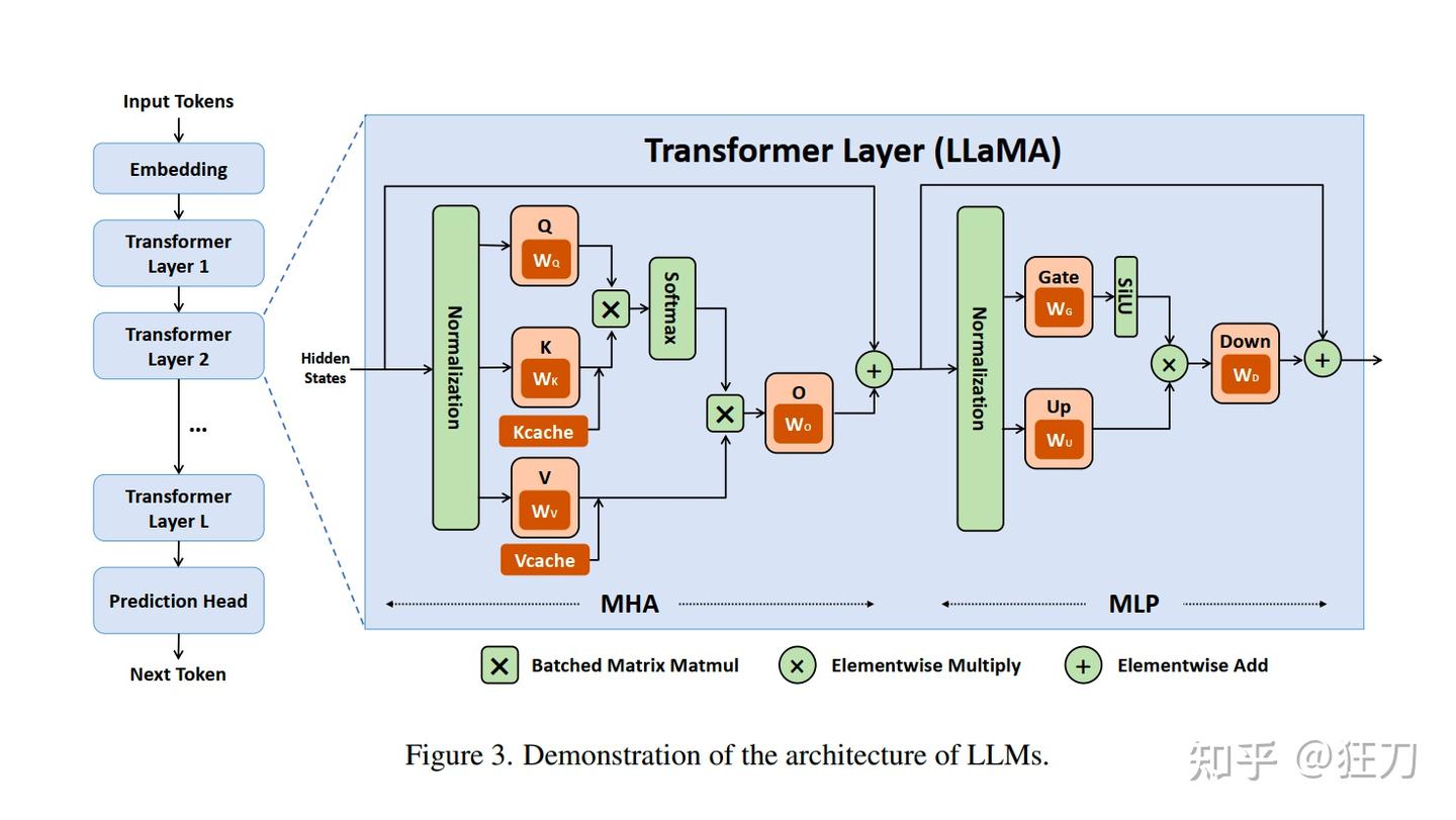
Prefill Stage Analysis

In the prefill stage, we process a batch of prompts with shape (b, s, h), where b is batch size, s is sequence length, and h is the hidden dimension.

1. Multi-Head Attention (MHA) Cost

The MHA block performs several key operations:

1. Q, K, V Projections: The input x of shape (b, s, h) is multiplied by three weight matrices (W_q, W_k, W_v), each of shape (h, h), to produce the Q, K, and V tensors.

   • Operation: A batched matrix multiplication (BMM) of shape (b*s, h) @ (h, h).
   • Compute (FLOPs): For each projection, this is approximately 2 * (b * s) * h * h = 2bsh^2. Total for all three is 6bsh^2. This is a classic dense matrix-matrix multiplication.
   • Memory (I/O): We read the input x and the weight matrix, and write the output (Q, K, or V).

2. Attention Scores (Q @ K^T): The Q tensor is multiplied by the transpose of the K tensor. To handle multiple heads, the tensors are reshaped. Per head, this is a matmul of shape (s, d_k) @ (d_k, s), where d_k = h / a (a = number of heads).

   • Compute (FLOPs): Summed across all heads, this is 2 * b * a * s * d_k * s = 2bs^2h.
   • Memory (I/O): This operation creates a large intermediate tensor of shape (b, a, s, s) for the attention scores. The s^2 term means this can consume a huge amount of memory for long sequences. This is the primary bottleneck that optimizations like FlashAttention target.

3. Attention Output (Scores @ V): The attention scores are multiplied by the V tensor. Per head, this is a matmul of shape (s, s) @ (s, d_k).

   • Compute (FLOPs): Summed across heads, this is 2 * b * a * s * s * d_k = 2bs^2h.

2. Feed-Forward Network (FFN) Cost

Modern FFNs (like Llama's SwiGLU) use three weight matrices (W_gate, W_up, W_down) to transform the MHA output. The intermediate dimension i is typically a multiple of h (e.g., 4h).

1. Up-Projection & Gate-Projection: The input (b, s, h) is multiplied by two separate weight matrices of shape (h, i).
   • Compute (FLOPs): 2 * (2 * b * s * h * i) = 4bsih. These are also dense matrix-matrix multiplications.
2. Down-Projection: The result of the element-wise operations is multiplied by a weight matrix of shape (i, h).
   • Compute (FLOPs): 2 * b * s * i * h = 2bsih.

Quantitative Breakdown

The following article provides an excellent table summarizing the compute and memory costs for each step.

Key Insights from the Prefill Analysis:

• Overall Complexity: The total time complexity for the prefill stage is O(s^2h + sh^2). The sh^2 term comes from the dense linear projections (both in MHA and FFN), while the s^2h term comes from the attention score calculations.
• Bottleneck: Whether the prefill stage is compute-bound or memory-bound depends on the hardware and the relative sizes of s and h. For very long sequences (s > h), the attention calculations (s^2h) can dominate. For models with very large hidden dimensions, the projections (sh^2) dominate. These large matrix-matrix multiplications generally have high arithmetic intensity and can effectively saturate the GPU's compute units.

Decode Stage Analysis (Auto-Regression)

The decode stage is where the performance characteristics change dramatically. Here, we generate one token at a time. The input is a single vector of shape (b, 1, h). However, to maintain context, we must attend to all L previously generated tokens. This is made efficient by the KV Cache, which stores the Key and Value tensors from all previous steps.

Let's analyze the cost for generating a single token when the context length is L.

1. MHA Block (Decode Step):

   • Q, K, V Projections: We only need to compute Q, K, V for the new token. The input shape is (b, 1, h). These are matrix-vector multiplications.
     • Compute (FLOPs): ~6bh^2.
   • Attention (Q @ K^T and Scores @ V): The new single-token query Q (shape b, 1, h) must attend to the entire Key cache K_cache (shape b, L, h). The resulting scores must then be applied to the Value cache V_cache (shape b, L, h). These are matrix-vector multiplications.
     • Compute (FLOPs): The two steps are each O(bLh). Total is ~4bLh.
     • Memory (I/O): This is the critical part. To perform this calculation, the entire KV cache, of size 2 * b * L * h * (bytes_per_element), must be read from HBM.

2. FFN Block (Decode Step):

   • The FFN block processes a single vector of shape (b, 1, h). All operations are matrix-vector multiplications.
   • Compute (FLOPs): ~4bih.

The performance of the decode stage is almost entirely dictated by the memory bandwidth required to read the large KV cache at every single step.

Let's read a resource that formalizes this analysis.

Key Insights from the Decode Analysis:

• Low Arithmetic Intensity: The decode step involves reading a large amount of data (the KV cache) to perform a relatively small number of computations. As the resource shows, the arithmetic intensity is proportional to (Ld + d^2) / (Ld + Lh + d^2), which is less than 1.
• Memory-Bound: Because the arithmetic intensity is so low, the decode stage is almost always memory-bound. The speed of token generation (inter-token latency) is limited not by how fast the GPU can compute, but by how fast it can stream the KV cache from HBM to the processing units. This is a fundamental concept in LLM serving performance.

Self-Check Exercise

Consider a decoder block with h=4096 and a=32 attention heads.

1. Prefill Stage: You are processing a prompt with s=512. Which operation is likely to have a higher compute cost (FLOPs): the QKV projections or the attention score (Q @ K^T) calculation?
2. Decode Stage: The model is generating the 2000th token (L=2000). Which operation likely dominates the wall-clock time for the MHA block: the QKV projections for the new token, or the attention calculation involving the KV cache? Why?

...

Answers:

1. Prefill Stage:

   • QKV Projections FLOPs: O(sh^2) -> 512 * 4096^2 -> ~8.5 * 10^9
   • Attention Scores FLOPs: O(s^2h) -> 512^2 * 4096 -> ~1.0 * 10^9
     The QKV projections have a higher compute cost in this scenario, as h is much larger than s.

2. Decode Stage:

   • The attention calculation involving the KV cache will dominate the wall-clock time.
   • Why: While the QKV projections for the new token are compute-intensive (O(h^2)), they are matrix-vector operations that operate on small inputs. The attention calculation, however, requires reading the entire KV cache for 2000 tokens from slow HBM. This massive data movement makes it memory-bound and the primary determinant of latency for each decoding step.

Conclusion

This lesson dove into the operational costs within a transformer's forward pass, providing the analytical tools to move beyond simple memory calculations.

Key Takeaways:

• Operations can be either compute-bound or memory-bound, a characteristic determined by their Arithmetic Intensity.
• The prefill stage involves large matrix-matrix multiplications (sh^2 and s^2h), which can have high arithmetic intensity and often become compute-bound.
• The autoregressive decode stage is dominated by matrix-vector operations that read from the large KV cache. This results in very low arithmetic intensity, making this phase fundamentally memory-bound.
• This dichotomy explains a core phenomenon in LLM serving: a fast time-to-first-token (TTFT), driven by the parallel, compute-bound prefill, followed by a slower, steady generation rate (inter-token latency or ITL), limited by the memory-bound decode step.

Preview of the Next Lesson:

We've now seen how critical the KV cache is to the performance of the decode stage. In the next lesson, we will focus entirely on it, learning to calculate the total KV cache size for a given model, batch size, and sequence length. This will complete the trifecta of VRAM consumers: model weights, activations, and the KV cache.