Estimating Optimization Benefits with Amdahl’s Law

Good to see you again. In the previous lesson, you established a precise performance vocabulary: choose a system boundary, distinguish service time from queueing delay, and use throughput, utilization, and Little’s Law consistently. Those measurements tell you where time is going. This lesson adds a decision tool for answering the next question: if we make one part faster, how much will the whole workload improve?

Amdahl’s Law is central to GPU and ML-infrastructure reasoning because local acceleration is rarely equal to end-to-end acceleration. A kernel can become ten times faster; a model server, training iteration, or user request often cannot. By the end, you should be able to calculate the maximum benefit of a proposed optimization, assess whether it is worth pursuing, and explain the result clearly in an interview or design review.

---

The central idea: optimize time, not an impressive-looking component

Imagine a workload takes $T_1$ seconds before an optimization. Some fraction of that baseline execution time can benefit from an enhancement; the rest cannot.

Let:

• $f$ = fraction of the original runtime affected by the improvement;
• $1-f$ = fraction unaffected;
• $k$ = speedup of the affected part itself;
• $S$ = overall end-to-end speedup.

Normalize the original runtime to one unit:

$$T_1=1$$

The unaffected part still costs:

$$1-f$$

The improved part used to cost $f$, but now it is $k$ times faster, so it costs:

$$\frac{f}{k}$$

Thus the new normalized runtime is:

$$T_{\text{new}}=(1-f)+\frac{f}{k}$$

Overall speedup is old time divided by new time:

$$S=\frac{T_1}{T_{\text{new}}}=\frac{1}{(1-f)+\frac{f}{k}}$$

This is the general form of Amdahl’s Law.

The implication is straightforward but powerful:

The benefit of an optimization depends on both its local speedup and the original fraction of total time it affects.

A 100x improvement in a 1% component is not a 100x faster system. Conversely, a modest improvement to a component responsible for most runtime can be highly valuable.

---

From a local optimization to an end-to-end estimate

Consider a training iteration that originally takes 1,000 ms:

Component	Baseline time	Fraction of total
Input pipeline and host preparation	100 ms	10%
GPU matrix multiplications	600 ms	60%
Other GPU kernels	150 ms	15%
Gradient synchronization	100 ms	10%
Miscellaneous overhead	50 ms	5%
Total	1,000 ms	100%

Suppose reduced precision and tensor-core-friendly kernels make the matrix multiplication portion 4x faster. The improved fraction is:

$$f=0.60$$

and the local speedup is:

$$k=4$$

Amdahl’s Law gives:

$$S=\frac{1}{(1-0.60)+\frac{0.60}{4}}=\frac{1}{0.40+0.15}=\frac{1}{0.55}\approx 1.82$$

So the whole training iteration can be at most about 1.82x faster, not 4x faster.

It is often clearer to convert that speedup back into time:

$$T_{\text{new}}=\frac{1000\text{ ms}}{1.82}\approx 550\text{ ms}$$

Or calculate directly from components:

$$T_{\text{new}}=100\text{ ms}+\frac{600\text{ ms}}{4}+150\text{ ms}+100\text{ ms}+50\text{ ms}=550\text{ ms}$$

The optimization saves 450 ms per iteration. That is substantial—but 400 ms of baseline work remains and becomes the new focus of performance analysis.

The maximum possible benefit

Now take the proposed optimization to its impossible but useful extreme: matrix multiplication takes zero time.

Mathematically, let:

$$k\to \infty$$

Then:

$$\frac{f}{k}\to 0$$

so the upper bound becomes:

$$S_{\max }=\frac{1}{1-f}$$

For the example where $f=0.60$:

$$S_{\max }=\frac{1}{1-0.60}=2.5$$

Even an infinitely fast matrix-multiplication component could make this iteration only 2.5x faster. Its time cannot go below the 400 ms spent elsewhere.

This is what makes Amdahl’s Law valuable before implementation: it can prevent months of work toward an objective that is mathematically impossible under the measured workload profile.

---

Parallelization is a special case

Amdahl’s Law applies to any improvement: a faster algorithm, a compiler optimization, quantization, an optimized library, improved storage, or a GPU kernel rewrite. Parallelization is simply a common special case.

Suppose a fraction $P$ of a program can be divided perfectly among $N$ processors. If all processors perform identical shares with no overhead, that fraction is accelerated by:

$$k=N$$

Substitute $k=N$ into the general equation:

$$S(N)=\frac{1}{(1-P)+\frac{P}{N}}$$

This is the standard strong-scaling form of Amdahl’s Law.

The assumptions matter:

• the problem size is fixed;
• the parallel portion divides evenly;
• processors are identical;
• communication and scheduling overhead are ignored;
• the serial portion does not grow.

The last three assumptions are usually optimistic for distributed AI systems. Still, the equation is an essential first estimate.

Suppose 95% of a fixed-size workload is ideally parallelizable:

$$P=0.95$$

With five processors:

$$S(5)=\frac{1}{0.05+\frac{0.95}{5}}=\frac{1}{0.24}\approx 4.17$$

With ten processors:

$$S(10)=\frac{1}{0.05+\frac{0.95}{10}}=\frac{1}{0.145}\approx 6.90$$

With 100 processors:

$$S(100)=\frac{1}{0.05+\frac{0.95}{100}}\approx 16.81$$

The theoretical ceiling, no matter how many processors are added, is:

$$S_{\max }=\frac{1}{1-0.95}=20$$

Doubling the processor count from 5 to 10 improves the parallel section by 2x, but it does not double the overall system speedup. The serial 5% stays fixed and increasingly dominates elapsed time.

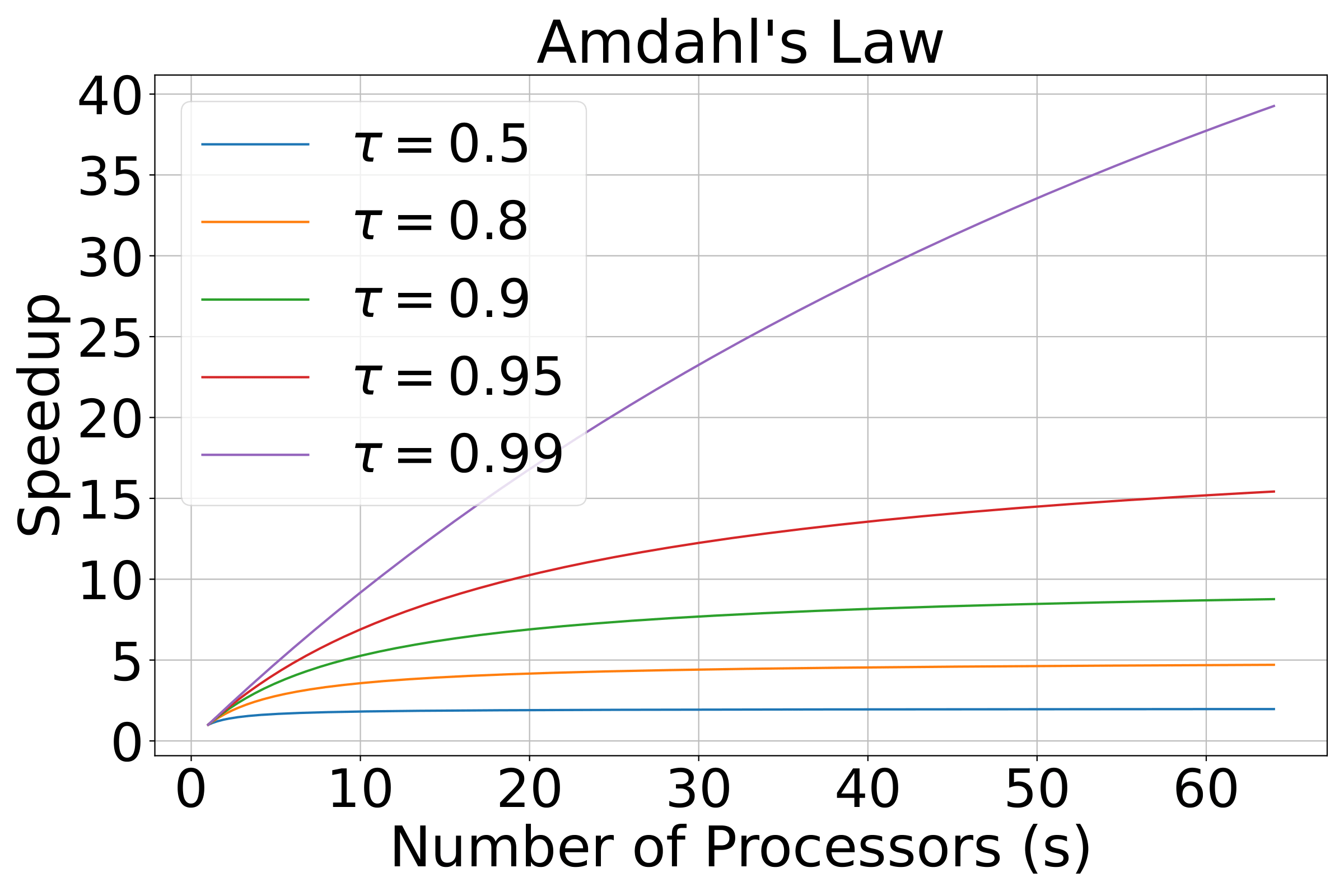
The graph captures two distinct design lessons:

1. Higher parallelizable fraction matters enormously.
   Moving from 90% to 99% parallelizable work changes the theoretical ceiling from 10x to 100x.

2. More processors eventually provide less value.
   For a fixed workload, extra resources chiefly accelerate a shrinking part of remaining execution time.

The normalized form can be convenient, but always return to actual milliseconds, dollars, and SLOs when making an engineering decision.

---

An LLM-serving example: accelerate decode, but quantify the user-visible gain

Amdahl’s Law is especially useful for LLM serving proposals. “We can make decoding faster” is not sufficient reasoning. First identify how much end-to-end time decode actually contributes under the target workload.

Suppose an LLM request has this no-queue timing profile:

Stage	Time
Gateway, validation, routing	40 ms
Scheduler waiting and batch formation	60 ms
Prompt prefill	300 ms
Autoregressive decode	900 ms
Token streaming and completion work	200 ms
End-to-end latency	1,500 ms

Assume an optimization improves decode throughput by 2x for this workload. The affected fraction is:

$$f=\frac{900}{1500}=0.60$$

The improvement factor is:

$$k=2$$

Then:

$$S=\frac{1}{0.40+\frac{0.60}{2}}=\frac{1}{0.70}\approx 1.43$$

New idealized end-to-end latency is:

$$T_{\text{new}}=\frac{1500\text{ ms}}{1.43}\approx 1050\text{ ms}$$

The result is a 1.43x speedup, or an approximately 30% latency reduction:

$$\frac{1500-1050}{1500}=0.30$$

This is a good improvement, but it is not “2x lower request latency.” The unoptimized 600 ms remains.

The absolute upper bound, even if decode became free, would be:

$$S_{\max }=\frac{1}{1-0.60}=2.5$$

So a sub-600 ms end-to-end latency target cannot be met by decode optimization alone. It requires reducing prefill, scheduler delay, network or gateway cost, output handling, or the amount of generated text.

Use the correct fraction for the decision

The affected fraction must be a fraction of time, not a fraction of code, requests, or tokens.

These are all different statements:

• “Decode is 60% of latency.”
  This can be used directly in Amdahl’s Law.

• “Decode has 60% of GPU FLOPs.”
  Potentially relevant, but not automatically a 60% time fraction.

• “60% of requests generate long answers.”
  Not a runtime fraction.

• “Decode runs in 60% of code paths.”
  Not necessarily a runtime fraction.

For a production decision, profile the representative traffic mix. A workload dominated by long generations may spend most of its time decoding; a workload with very long prompts and short answers may be prefill-dominated. The expected value of a decode optimization is therefore workload-dependent.

---

A practical optimization workflow

Amdahl’s Law is not a replacement for profiling. It is a disciplined way to use profiling evidence.

1. Define the objective and measurement boundary

Be explicit about what you are trying to improve:

• training iteration time;
• time to first token;
• inter-token latency;
• full request completion latency;
• total cluster cost per training token;
• throughput at a fixed latency target.

A kernel improvement may strongly improve one objective but barely affect another. For example, an optimization targeting decode execution may improve inter-token latency while having a limited effect on time to first token, which is mainly determined by queueing and prompt prefill.

2. Establish a representative baseline

Measure component times on the workload that matters:

$$T_1=\sum _i{T}_i$$

If you are evaluating a training change, profile a stable iteration after warm-up. If you are evaluating serving, use a representative distribution of prompt lengths, output lengths, request arrival patterns, and batching conditions.

Amdahl’s Law is only as credible as the baseline decomposition.

3. State exactly what the proposed change affects

Say, for example:

“This kernel fusion reduces the 180 ms activation-memory traffic component, which is 30% of a 600 ms iteration, by approximately 2x.”

That statement gives:

$$f=0.30,k=2$$

and therefore:

$$S=\frac{1}{0.70+\frac{0.30}{2}}\approx 1.18$$

The best predicted outcome is an 18% end-to-end speedup. Whether that is worth engineering effort depends on cost, risk, expected reuse, and the performance requirement—not on the fact that the kernel itself is 2x faster.

4. Calculate both predicted and maximum gains

Always calculate:

$$S=\frac{1}{(1-f)+\frac{f}{k}}$$

and:

$$S_{\max }=\frac{1}{1-f}$$

The first answers, “What does this particular proposed improvement buy us?” The second answers, “Could this category of optimization ever meet our goal?”

5. Re-profile after the change

An optimization shifts the bottleneck. The 600 ms matrix-multiplication component in the earlier example shrank to 150 ms, making previously secondary components relatively more important. Repeat the cycle:

$$\text{Measure}\to \text{estimate}\to \text{optimize}\to \text{measure again}$$

This is the core of NVIDIA’s assess–parallelize–optimize–deploy approach.

---

Reality check: why measured scaling can be worse than Amdahl predicts

Amdahl’s Law usually provides an optimistic upper bound. Real GPU and distributed systems may scale worse because the assumption of a perfectly accelerated component fails.

For ideal parallel scaling, the model says:

$$T_{\text{new}}=(1-P)+\frac{P}{N}$$

A more realistic normalized model includes overhead that changes with processor count:

$$T_{\text{new}}=(1-P)+\frac{P}{N}+O(N)$$

where $O(N)$ represents effects such as:

• synchronization barriers;
• collective communication;
• NVLink, PCIe, or network transfers;
• load imbalance and stragglers;
• kernel-launch and scheduling overhead;
• contention for memory bandwidth;
• nonuniform data partitioning.

You do not need an exact analytic formula for $O(N)$ to apply Amdahl’s reasoning. You can instead use the observed effective speedup of the component.

For example, suppose eight GPUs improve an operation only 5x rather than the ideal 8x because of all-reduce communication. Use:

$$k=5$$

not:

$$k=8$$

The key modeling rule is:

Use $k$ as the speedup you can realistically achieve for the affected portion, including the costs needed to obtain that speedup.

This matters in distributed training. Tensor parallelism may reduce compute per GPU, but it introduces communication on critical paths. Data parallelism may scale batch processing, but gradient synchronization can become a major component. Later modules will give you tools to estimate those communication costs explicitly.

---

Common mistakes in interviews and design reviews

Confusing the improved fraction with the remaining fraction

If 80% of time is accelerated, then:

$$f=0.80$$

and the untouched fraction is:

$$1-f=0.20$$

The upper bound is:

$$S_{\max }=\frac{1}{0.20}=5$$

A common error is to use $1/0.80$, which reverses the meaning.

Treating local speedup as system speedup

If a kernel is 10x faster but represents 10% of baseline runtime:

$$S=\frac{1}{0.90+\frac{0.10}{10}}=\frac{1}{0.91}\approx 1.10$$

The system is only about 10% faster.

Adding speedups directly

If one component is 2x faster and another is 3x faster, the total system is not “5x faster.” Convert each baseline component to its new time, sum those times, and divide baseline total time by the result.

For non-overlapping baseline fractions $f_1$ and $f_2$, with local speedups $k_1$ and $k_2$:

$$T_{\text{new}}=(1-f_1-f_2)+\frac{f_1}{k_1}+\frac{f_2}{k_2}$$

Then:

$$S=\frac{1}{T_{\text{new}}}$$

This only works when the fractions are measured on the same baseline and do not overlap. If two optimizations affect the same time interval, model their interaction rather than double-counting it.

Using a microbenchmark fraction instead of end-to-end time

A kernel might be 80% of GPU execution time but only 30% of end-to-end request time because queueing, serialization, CPU work, and network stages are outside the GPU. Use the boundary that matches the objective.

Applying Amdahl’s Law naively to queueing latency

The previous lesson distinguished service time from queueing delay:

$$W=W_q+S$$

Amdahl’s Law models a fixed workload’s execution time. In a loaded service, reducing service time also lowers utilization, which can sharply reduce queueing delay. Thus an optimization can yield a bigger improvement in observed end-to-end latency than an Amdahl calculation based on a fixed queue-inclusive latency might suggest.

That does not violate Amdahl’s Law. It means the system’s operating point changed: faster service reduced congestion. For a loaded service, combine Amdahl-style service-time estimates with utilization, queue-depth, and tail-latency analysis rather than treating one equation as a complete queueing model.

---

Strong scaling versus scaled workloads

This lesson’s use of Amdahl’s Law is strong scaling: a fixed task completes faster as more resources are added.

For example:

• train the same model on the same token count faster;
• serve the same prompt and generate the same output faster;
• process the same dataset in less elapsed time.

There is another valid question: as more GPUs become available, can we solve a larger problem in roughly the same time? That is the motivation for Gustafson’s Law and weak scaling. It is relevant to training larger models, raising sequence length, or processing more data.

However, it does not erase Amdahl’s Law for a fixed latency or fixed-workload objective. If the question is, “Will adding GPUs make this specific job finish within its deadline?” Amdahl’s Law remains the appropriate starting point.

---

A concise answer pattern for system-design interviews

When asked whether an optimization is worthwhile, structure the answer as follows:

1. Name the boundary and objective.
   “I will evaluate stable training-iteration time,” or “I will evaluate model-admission-to-final-token latency.”

2. Profile the baseline.
   “The targeted stage is 55% of baseline time.”

3. Estimate the local speedup realistically.
   “The new implementation is expected to make that stage 2.5x faster after communication overhead.”

4. Apply Amdahl’s Law.

   $$S=\frac{1}{0.45+\frac{0.55}{2.5}}\approx 1.49$$

5. State the implication in operational terms.
   “The best estimate is a 1.49x overall speedup, reducing a 900 ms iteration to about 604 ms.”

6. State the ceiling and next validation step.

   $$S_{\max }=\frac{1}{0.45}\approx 2.22$$

   “Even perfect acceleration of this stage cannot exceed 2.22x. I would implement a benchmark or controlled canary, then re-profile because synchronization or input work may become the bottleneck.”

This demonstrates more than formula recall: it shows disciplined performance reasoning.

---

Key takeaways

• Amdahl’s Law estimates overall speedup from an optimization affecting a fraction $f$ of baseline runtime:

$$S=\frac{1}{(1-f)+\frac{f}{k}}$$

where $k$ is the speedup of the improved portion.

• The absolute ceiling for accelerating that portion is:

$$S_{\max }=\frac{1}{1-f}$$

• Ideal parallelization across $N$ processors is a special case:

$$S(N)=\frac{1}{(1-P)+\frac{P}{N}}$$

• Measure $f$ as a time fraction within the exact system boundary and workload relevant to the decision.

• Use Amdahl’s Law before implementation to set realistic targets, but use profiling after implementation to capture communication, overhead, bottleneck shifts, and queueing effects.

• For AI systems, distinguish an improvement to a kernel, GPU execution, training iteration, TTFT, decode latency, and full user-visible request latency. Their affected fractions can differ dramatically.

Next, you will examine arithmetic intensity and the roofline model. Amdahl’s Law tells you whether improving a component can matter end-to-end; roofline analysis helps identify why that component is limited—by compute throughput or memory bandwidth—and therefore which optimization is plausible.