Analyzing Performance Metrics with Little’s Law

Hello, and welcome to the first module of this course. We will begin with the performance vocabulary that underlies GPU systems, distributed training, and LLM serving: latency, throughput, utilization, and concurrency. These quantities are easy to name but frequently misinterpreted in system-design discussions—especially when batching, queues, and multiple GPUs are involved.

This lesson develops a calculation-first framework for moving from timing data to operational conclusions: how busy a resource is, how much work is concurrently in the system, and whether latency is dominated by work itself or by waiting. These tools will recur throughout the course, from CUDA kernels to distributed training and production LLM services.

---

Four quantities, one carefully chosen boundary

Before calculating anything, draw a boundary around the system or resource you mean to analyze. It might be:

• an API request from admission to final response;
• a model-server replica;
• a GPU execution queue;
• a database connection pool;
• an entire multi-stage service.

The same request can have different latency and concurrency depending on that boundary. That is not a contradiction—it is the point of choosing one explicitly.

The core quantities are:

Quantity	Symbol	Meaning	Typical unit
Latency / response time	$W$ or $T$	Time from entering the chosen boundary to leaving it	ms, s
Service time	$S$	Time a resource actively spends processing work, excluding queueing	ms, s
Queueing delay	$W_q$	Time waiting before service begins	ms, s
Throughput	$X$	Rate of completed admitted work	requests/s, tokens/s
Arrival rate	$\lambda$	Rate at which work enters the boundary	requests/s
Utilization	$\rho$	Fraction of available service capacity that is busy	fraction or percent
In-flight concurrency	$L$ or $N$	Average number of requests currently inside the boundary	requests

For a request that visits one queue and one worker:

$$W=W_q+S$$

This decomposition is operationally useful:

• If $S$ dominates, reduce the amount of work or make the execution faster.
• If $W_q$ dominates, the resource is congested, scheduling is poor, traffic is bursty, or capacity is insufficient.

Do not call every delay “latency” and stop there. A 500 ms response could mean 490 ms of computation, or 10 ms of computation plus 490 ms waiting in a queue. The remedies are completely different.

---

Throughput is completed work, not “how fast one request feels”

Throughput is the long-run completion rate:

$$X=\frac{\text{number of completed jobs}}{\text{measurement duration}}$$

If a model-serving replica completes 18,000 requests over a five-minute steady-state interval:

$$X=\frac{18,000}{300}=60\text{requests/s}$$

For LLM serving, it is common—and necessary—to track at least two throughputs:

• Request throughput, e.g. $60$ requests/s.
• Token throughput, e.g. $9,000$ generated tokens/s.

Neither replaces the other. Request throughput reflects user-facing capacity, while token throughput better reflects model work for variable-length generations. A service can maintain a similar request rate while token throughput changes substantially if users begin requesting longer answers.

In a stable, lossless system over a sufficiently long interval:

$$X\approx \lambda$$

That is, admitted work eventually completes, so rate in equals rate out. But there are important exceptions:

• During a short ramp-up or ramp-down interval, arrivals and completions need not match.
• With admission control, rejection, or dropped requests, offered arrival rate differs from admitted arrival rate.
• With retries, a “request” may enter downstream stages more than once.
• In a streaming LLM response, request completion rate and token emission rate describe different units of work.

For capacity and Little’s Law, use the rate associated with the exact boundary and the population you are measuring. If 150 requests/s arrive at a gateway but only 120 requests/s are admitted to the model server, use $120$ requests/s when analyzing the model-server queue.

---

Latency: use the right timestamp pair

Latency is simply a difference between timestamps—but the timestamps must match the question.

For an ordinary request:

$$W=t_{\text{completion}}-t_{\text{admission}}$$

For a stage within a pipeline:

$$S_{\text{stage}}=t_{\text{stage end}}-t_{\text{stage start}}$$ $$W_{q,\text{stage}}=t_{\text{stage start}}-t_{\text{stage arrival}}$$

In a production system, define timestamp ownership precisely. For example, “gateway arrival” might mean load balancer receipt, while “model admission” might mean the scheduler has accepted the request into a batchable queue. Those are both defensible boundaries, but they report different performance.

For LLM interactions, token streaming adds further user-relevant latency boundaries:

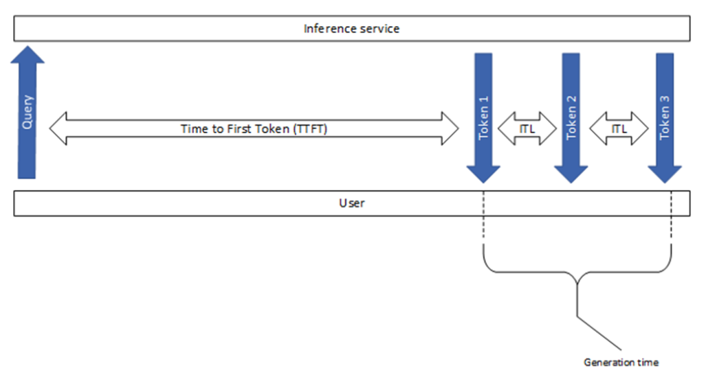
The detailed prefill/decode mechanics behind these LLM-specific measures come later. For now, notice the general rule: a latency metric must state its start event and end event. “Model latency” without those boundaries is not a useful metric.

Measure distributions, not only averages:

• Mean latency supports aggregate capacity calculations.
• p50 describes a typical request.
• p95/p99 show the tail experience and often reveal queueing, imbalance, long prompts, or noisy-neighbor effects.
• Maximum latency is usually too sensitive to isolated failures to summarize normal behavior.

A service can have an acceptable mean while violating a p99 objective badly. Nevertheless, Little’s Law uses a mean latency and an average in-flight count—not p99 latency.

---

Utilization: how much of a resource is actually busy

Utilization is the fraction of a resource’s available time spent doing work:

$$\rho =\frac{\text{busy time}}{\text{available time}}$$

If a GPU is executing kernels for 42 seconds during a 60-second observation window:

$${\rho }_{\text{GPU}}=\frac{42}{60}=0.70=70\%$$

For a single server that handles one request at a time, utilization can also be estimated from throughput and mean service time:

$$\rho =XS$$

For $c$ homogeneous workers, each capable of handling one request at a time:

$$\rho =\frac{XS}{c}$$

Equivalently, if each worker’s mean service rate is $\mu =1/S$:

$$\rho =\frac{X}{c\mu }$$

The denominator, $c\mu$, is the system’s idealized service capacity. A stable queue requires:

$$\rho <1$$

At $\rho \ge 1$, arrivals require at least as much capacity as the workers can provide. Queues then grow until some external mechanism intervenes: a timeout, rejection, client backoff, memory exhaustion, or system failure.

The important systems lesson is subtler than “keep utilization below 100%.” Queueing delay often rises sharply well before 100% because real workloads are variable:

• arrivals occur in bursts;
• request sizes differ;
• some requests are unusually slow;
• scheduling and load balancing are imperfect;
• garbage collection, communication stalls, or kernel variation create pauses.

Thus, a system designed to sit at 95–99% sustained utilization is usually designed to have poor tail latency. The appropriate headroom depends on workload variability and the latency objective; there is no universal safe percentage.

One caution for GPU and LLM systems: direct busy-time utilization is always meaningful if defined clearly, but the simple formula $\rho =XS$ needs care when a GPU processes a batch of requests simultaneously. A request may share GPU kernel execution with many others, so there may not be a clean per-request exclusive service time $S$. In that setting:

• measure GPU utilization as busy GPU time divided by elapsed time;
• measure request throughput and token throughput separately;
• use empirical service curves under representative batch sizes rather than pretending each request owns an independent GPU interval.

---

Little’s Law: turning latency into concurrency

Little’s Law connects the average number of items inside a system to throughput and average latency:

$$L=XW$$

where:

• $L$ is average in-flight concurrency;
• $X$ is throughput through the chosen boundary;
• $W$ is mean time spent inside that boundary.

It is unusually general. It does not require Poisson arrivals, exponential service times, FIFO scheduling, or a single server. It does require that the system be sufficiently stable over the measurement interval: work should not accumulate indefinitely, and the observed averages should be meaningful.

The units provide a valuable sanity check:

$$\frac{\text{requests}}{\text{s}}\times \text{s}=\text{requests}$$

Suppose a stable service sustains $120$ requests/s and has mean end-to-end latency of $150$ ms:

$$L=120\times 0.150=18$$

On average, 18 requests are in flight: some executing, some waiting, perhaps some traversing network or serialization stages—depending on the boundary.

If you separately know mean service time is $20$ ms, then mean queueing delay is:

$$W_q=W-S=150\text{ ms}-20\text{ ms}=130\text{ ms}$$

Little’s Law can be applied to the queue alone:

$$L_q=X{W}_q$$ $$L_q=120\times 0.130=15.6$$

So approximately $15.6$ requests are waiting, on average. The remaining average work in service is:

$$L_{\text{service}}=XS=120\times 0.020=2.4$$

The accounting checks out:

$$L_q+L_{\text{service}}=15.6+2.4=18$$

This is a powerful diagnosis. The end-to-end latency is 150 ms, but only 20 ms is active service. Faster compute might help, but this system’s immediate problem is evidently queueing.

---

Worked capacity calculation from workload timing data

Consider a model-serving fleet with four identical request workers. Over a stable 10-minute interval, monitoring reports:

• completed requests: $72,000$;
• mean request latency from model admission to final response: $150$ ms;
• mean active worker service time per request: $20$ ms;
• no rejected requests during the interval.

1. Compute throughput

$$X=\frac{72,000}{600}=120\text{requests/s}$$

2. Compute average in-flight concurrency

Convert milliseconds to seconds:

$$W=150\text{ ms}=0.150\text{ s}$$

Then apply Little’s Law:

$$L=XW=120\times 0.150=18$$

There are 18 requests in the model-serving boundary on average.

3. Compute worker utilization

There are $c=4$ workers, each with mean service time $S=0.020$ s:

$$\rho =\frac{XS}{c}=\frac{120\times 0.020}{4}=0.60$$

Each worker is busy about 60% of the time, on average.

The implied per-worker service rate is:

$$\mu =\frac{1}{S}=\frac{1}{0.020}=50\text{requests/s}$$

Total idealized service capacity is:

$$c\mu =4\times 50=200\text{requests/s}$$

At 120 requests/s, the offered load is $120/200=60\%$, matching the utilization calculation.

4. Separate queueing from service

$$W_q=W-S=0.150-0.020=0.130\text{ s}$$ $$L_q=X{W}_q=120\times 0.130=15.6$$

Interpretation:

• about $2.4$ requests are actively being served across the four workers;
• about $15.6$ requests are waiting, on average;
• mean latency is queueing-dominated despite moderate aggregate utilization.

That last point should prompt investigation rather than an automatic conclusion. Possible explanations include bursty arrivals, unequal worker load, serial stages hidden within “service,” admission/scheduling delay, or a mismatch between the modeled boundary and the timestamps used.

---

Applying the same logic to LLM serving

Suppose an LLM service runs for 60 seconds under a representative workload and observes:

• 300 completed requests;
• 36,000 output tokens generated;
• 8 s mean request latency from admission to final token;
• 75% measured GPU busy utilization.

First, report both rates:

$$X_{\text{request}}=\frac{300}{60}=5\text{requests/s}$$ $$X_{\text{output token}}=\frac{36,000}{60}=600\text{tokens/s}$$

Now use request throughput—not output token throughput—for request concurrency:

$$L_{\text{requests}}=X_{\text{request}}W=5\times 8=40$$

The service has, on average, 40 admitted requests in flight.

This does not mean that 40 requests are executing one per GPU. Some may be awaiting prefill, some may be included in a batch, and some may be awaiting their next decode step. The average is still useful: it informs queue capacity, scheduler limits, cancellation behavior, and memory budgeting. But interpretation requires knowledge of the serving engine.

It would be incorrect to compute request utilization as $5\times 8=40$. That quantity is concurrency, not utilization. It would also be incorrect to infer that a 75% busy GPU has 25% spare request capacity: the next requests may have longer prompts, larger KV-cache footprints, or poor batch compatibility.

For LLM serving, use the following mental separation:

Question	Appropriate quantity
How many user requests are active or queued?	$L=X_{\text{request}}W$
How much model generation is happening?	output token throughput
How busy is the GPU?	measured GPU busy-time utilization
Is queueing hurting users?	queue time plus TTFT and tail latency
Can another request fit in memory?	KV-cache and batch-capacity analysis

We will later connect these metrics to prefill, decode, continuous batching, KV-cache capacity, and the distinct behavior of token streaming.

---

A reliable measurement workflow

When given a dashboard, trace, or interview-style timing table, work through this sequence.

1. Choose the system boundary.
   State where a request enters and leaves. Do not combine gateway arrival rate with GPU-only latency.

2. Choose a steady-state interval.
   Exclude deployment warm-up, model loading, synthetic-test ramp phases, and outages unless the goal is explicitly to analyze them.

3. Compute throughput from completions.

   $$X=\frac{C}{\Delta t}$$

   where $C$ is completions in duration $\Delta t$.

4. Compute mean latency from matching request timestamps.
   Use the same boundary as throughput. Retain p50, p95, and p99 alongside the mean.

5. Estimate in-flight work with Little’s Law.

   $$L=XW$$

6. Compute utilization at a specific resource.
   Prefer direct busy-time measurement:

   $$\rho =\frac{\text{busy time}}{\text{available time}}$$

   Or use $\rho =XS/c$ only where $S$ represents well-defined per-job service demand on $c$ equivalent servers.

7. Validate using independent evidence.
   If Little’s Law predicts $L=40$, compare it with time-averaged in-flight gauges, scheduler queue depth plus active requests, or trace-derived concurrency. A large discrepancy usually indicates mismatched boundaries, unstable traffic, dropped work, incorrect units, or a biased sampling method.

Two common mistakes are worth making explicit:

• Mixing milliseconds and seconds.
  At $1,000$ requests/s and $50$ ms latency:

  $$L=1,000\times 0.050=50$$

  not 50,000.

• Using p99 latency in Little’s Law.

  $$L=X\times \text{mean latency}$$

  Little’s Law relates average occupancy to average time. Tail latency is essential for SLOs, but it does not directly substitute into this equation.

---

Closed-loop clients and “think time”

A final boundary issue matters for load testing and interactive applications. A closed-loop client alternates between issuing a request and waiting, perhaps with think time or pacing:

$$\text{cycle time}=\text{response time}+\text{think time}+\text{pacing}$$

For this broader client-loop boundary:

$$N_{\text{clients}}=X\times \left(W_{\text{response}}+W_{\text{think}}+W_{\text{pacing}}\right)$$

Think time belongs in the equation only if your boundary includes the client loop. It does not belong in server-side in-flight concurrency.

This distinction explains why a test may need 100 virtual users to produce 20 requests/s while the server itself has only 10 requests in flight. The remaining users are reading, waiting, or pacing before their next request.

---

Key takeaways

• Latency is time inside a specified boundary; distinguish active service time from queueing delay.
• Throughput is the completion rate of a well-defined unit: requests, tokens, jobs, or batches.
• Utilization is the busy fraction of a particular resource. For $c$ homogeneous one-job-at-a-time workers, $\rho =XS/c$.
• Little’s Law connects mean concurrency, throughput, and mean latency: $$L=XW$$
• Stable systems have admitted arrival rate approximately equal to completion throughput; rejected, retried, or ramping traffic needs more careful accounting.
• In batched LLM inference, request concurrency, token throughput, and GPU utilization are all necessary—but they are not interchangeable.

Next, we will use Amdahl’s Law to estimate the maximum end-to-end benefit of an optimization. That will provide a disciplined way to answer a common infrastructure question: if we accelerate one part of the workload, how much faster can the whole system actually become?