Using Arithmetic Intensity and the Roofline Model to Classify AI Workloads

Welcome back. In the last lesson, you used Amdahl’s Law to decide whether accelerating a component can materially improve an end-to-end training iteration or serving request. That analysis begins with measured time fractions. This lesson moves one level deeper: for a GPU kernel that matters, what fundamentally limits its speed?

The central tool is the roofline model. It relates the computation performed by an operation to the bytes it must move, then compares that ratio with the GPU’s own compute-to-bandwidth ratio. By the end, you should be able to estimate an AI kernel’s arithmetic intensity, place it on a roofline, classify it as compute-bound or memory-bandwidth-bound, and propose an optimization that matches the bottleneck.

---

Two resources, one execution time

Consider a GPU kernel that performs $W$ floating-point operations and transfers $Q$ bytes across a particular memory interface—usually GPU high-bandwidth memory (HBM).

Two lower bounds constrain its execution time:

$$T_{\text{compute}}=\frac{W}{P_{\text{peak}}}$$ $$T_{\text{memory}}=\frac{Q}{BW}$$

where:

• $P_{\text{peak}}$ is the relevant peak compute throughput, in FLOPs/s;
• $BW$ is the relevant memory bandwidth, in bytes/s;
• $W$ is total floating-point work;
• $Q$ is bytes read and written.

If memory transfers and arithmetic overlap well, an optimistic runtime estimate is:

$$T_{\text{kernel}}\gtrsim \max \left(T_{\text{compute}},T_{\text{memory}}\right)$$

The larger term determines the likely bottleneck:

• If $T_{\text{memory}}>T_{\text{compute}}$, the kernel is memory-bandwidth-bound. Compute units must wait for data from HBM.
• If $T_{\text{compute}}>T_{\text{memory}}$, it is compute-bound. Data arrives fast enough, but arithmetic throughput is the limiting resource.

This is not merely terminology. It tells you what kind of optimization has a plausible payoff:

Likely limiter	Usually promising	Usually not sufficient by itself
Memory bandwidth	Reduce HBM traffic; reuse data; fuse kernels; improve access efficiency	Buying more FLOPs/s
Compute throughput	Use efficient matrix multiplication; compatible reduced precision; improve tensor-core utilization	Reducing a small amount of memory traffic
Latency / insufficient parallelism	Increase useful concurrency; reduce launch overhead; improve work granularity	Applying a bandwidth-only or FLOP-only model

The last row is important. Roofline analysis assumes enough work is available to keep the GPU busy. A tiny kernel can have high arithmetic intensity but still run slowly because there are too few thread blocks or too much fixed overhead. The roofline is therefore a first-order throughput model, not a complete explanation for every slowdown.

---

Arithmetic intensity: FLOPs earned per byte moved

The quantity that connects algorithm behavior with hardware is arithmetic intensity:

$$I=\frac{W}{Q}$$

Its units are FLOPs per byte.

Arithmetic intensity answers:

For each byte brought across the bottleneck interface, how much numerical work does this operation obtain from it?

A low-intensity operation consumes data and does very little with it. An elementwise activation is the classic case: load a value, apply a small operation, write a result. A high-intensity operation reuses values many times, as a large matrix multiplication does.

The hardware has a corresponding critical intensity:

$$I_{\text{crit}}=\frac{P_{\text{peak}}}{BW}$$

This is the intensity required to keep the compute hardware fully supplied.

The classification rule follows directly:

$$I<I_{\text{crit}}⟹\text{memory-bandwidth-bound}$$ $$I>I_{\text{crit}}⟹\text{compute-bound}$$

At the crossover point, $I=I_{\text{crit}}$, compute time and memory time are equal. This point is called the roofline knee.

The same relationship can be written as a throughput ceiling:

$$P_{\text{roof}}=\min \left(P_{\text{peak}},I\times BW\right)$$

When intensity is low, the achievable FLOP rate increases linearly with intensity because memory bandwidth is the ceiling. Once the kernel reaches peak compute throughput, more intensity cannot improve performance through this model—the curve becomes flat.

---

Reading a roofline plot

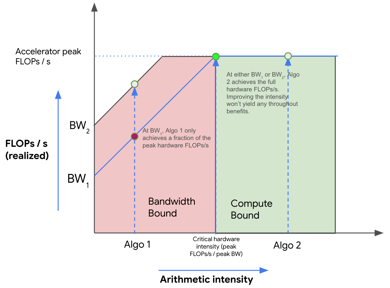
The roofline image makes several ideas visible at once:

1. The horizontal axis is arithmetic intensity.
   Moving right means obtaining more computation per byte transferred.

2. The vertical axis is achievable compute throughput.
   A kernel’s observed FLOPs/s cannot exceed the roofline appropriate to its precision and hardware path.

3. The diagonal portion is bandwidth-bound.
   Here:

   $$P_{\text{roof}}=I\times BW$$

   Increasing intensity or increasing bandwidth can improve performance.

4. The flat portion is compute-bound.
   Here:

   $$P_{\text{roof}}=P_{\text{peak}}$$

   More HBM bandwidth does not help this operation in the simplified model. A higher compute ceiling or a more efficient compute implementation might.

5. Bandwidth improvements matter only to the left of the knee.
   In the image, moving from BW1 to BW2 lifts the diagonal bandwidth roof. But it does not raise the flat compute roof. This distinction matters when comparing accelerators: a GPU with substantially more peak FLOPs but similar HBM bandwidth may make a low-intensity workload more bandwidth-bound.

A useful mental model is that a roofline is defined by a particular hardware interface and compute engine. For most single-GPU AI-kernel analysis, that interface is HBM and the compute engine is the relevant FP32, BF16, FP8, or INT8 execution path. Later, when training is distributed, the same logic will apply to NVLink and network links—except the bytes will be transferred between accelerators rather than between HBM and compute cores.

---

Worked example: a transformer linear layer

A transformer linear layer can be represented as a matrix multiplication:

$$X[B,D]\times W[D,F]\to Y[B,F]$$

where:

• $B$ is the number of token rows processed together;
• $D$ is the input or hidden dimension;
• $F$ is the output dimension, often the MLP expansion dimension;
• all tensors are BF16 for this simplified analysis.

A multiply-accumulate is conventionally counted as two FLOPs: one multiplication and one addition. Therefore, the operation count is approximately:

$$W=2BDF$$

Assume each BF16 element occupies two bytes and that $X$, $W$, and $Y$ are each transferred once to or from HBM. The byte traffic is:

$$Q=2BD+2DF+2BF$$

Thus arithmetic intensity is:

$$I=\frac{2BDF}{2BD+2DF+2BF}=\frac{BDF}{BD+DF+BF}$$

A representative H100-style roofline

Use an ideal dense BF16 tensor-core peak of:

$$P_{\text{peak}}=989\times 10^{12}\text{ FLOPs/s}$$

and HBM bandwidth of:

$$BW=3.35\times 10^{12}\text{ bytes/s}$$

The critical intensity is:

$$I_{\text{crit}}=\frac{989\times 10^{12}}{3.35\times 10^{12}}\approx 295\text{ FLOPs/byte}$$

Now consider a linear layer with:

$$D=F=8192$$

First use $B=128$ token rows.

$$I=\frac{128\times 8192\times 8192}{128\times 8192+8192\times 8192+128\times 8192}\approx 124\text{ FLOPs/byte}$$

Since:

$$124<295$$

the operation is predicted to be memory-bandwidth-bound.

The two idealized time limits make this concrete:

$$T_{\text{compute}}=\frac{17.18\times 10^9}{989\times 10^{12}}\approx 17.4\text{ microseconds}$$ $$T_{\text{memory}}=\frac{138.4\times 10^6}{3.35\times 10^{12}}\approx 41.3\text{ microseconds}$$

Memory traffic takes longer, so the idealized runtime is bounded below by roughly 41 microseconds.

Now raise the token-row batch to $B=512$:

$$I\approx 455\text{ FLOPs/byte}$$

Now:

$$455>295$$

so the same layer becomes compute-bound under this model.

Token rows processed together	Arithmetic intensity	Compute-time bound	HBM-time bound	Predicted limiter
$128$	$124$ FLOPs/byte	$17.4$ microseconds	$41.3$ microseconds	HBM bandwidth
$512$	$455$ FLOPs/byte	$69.5$ microseconds	$45.1$ microseconds	Compute throughput

The key change is not the layer’s dimensions or the GPU. It is reuse of the weight matrix. With more rows in $X$, each loaded weight participates in more dot products. The FLOP count rises with $B$, while the large $D\times F$ weight matrix is still loaded only once in the simplified model.

When $B$ is small relative to $D$ and $F$, the weight matrix dominates byte traffic. The expression becomes approximately:

$$I\approx B$$

for BF16 matrix multiplication. This is why the number of tokens processed together is such an important performance variable.

---

Why this predicts LLM training and serving behavior

A single LLM is not one roofline point. It is a sequence of kernels with different arithmetic intensities, memory-access patterns, and hardware ceilings. Analyze the important stages separately.

High-intensity work: large matrix multiplication

Dense transformer projections and MLP layers contain large matrix multiplications. During training, or during prompt prefill with enough tokens processed together, these operations can have high arithmetic intensity and become compute-bound.

For such kernels, plausible levers include:

• using a precision and layout that reach the intended matrix-multiply engine;
• choosing sufficiently efficient matrix dimensions and tiling;
• increasing useful token-level batching when latency and memory allow;
• improving tensor-core utilization.

The point is not simply “use lower precision.” Reduced precision changes both the available compute ceiling and bytes moved, so it changes the roofline itself. The actual result must still be modeled and measured.

Low-intensity work: elementwise operations and reductions

Operations such as activations, residual additions, normalization, and many reductions often do a handful of FLOPs per tensor element while reading and writing that element. Their arithmetic intensity is intrinsically low.

For example, a simple activation may read one value, do one comparison or arithmetic operation, and write one value. Even before counting indexing and instruction overhead, it has little opportunity to reuse data from HBM.

These operations are commonly bandwidth-bound. Useful strategies often include:

• kernel fusion, such as combining a bias, activation, and residual update so intermediate tensors are not written to HBM and read back;
• avoiding unnecessary casts, copies, or materialized intermediates;
• ensuring efficient, contiguous access patterns;
• improving reuse through an algorithm or layout change.

Kernel fusion is especially instructive: it may not reduce the mathematical FLOPs at all, but it can reduce $Q$, raising arithmetic intensity:

$$I=\frac{W}{Q}$$

That can deliver a real end-to-end improvement even when a profiler reports a modest FLOP rate. A memory-bound kernel need not exhibit high FLOP utilization to be performing well—it may be close to saturating HBM bandwidth instead.

Decode: why small batches tend to be bandwidth-bound

Autoregressive decode generates one token per sequence per step. If only a small number of sequences are active, a projection effectively resembles a matrix-vector multiply or a very skinny matrix multiplication. The large weight matrix must be streamed, but it is reused by only a small number of token rows.

That means low $B$, low intensity, and usually a bandwidth-bound regime.

Continuous batching in a serving system changes this. By grouping more active sequences into a decode step, it increases the effective $B$, enabling greater weight reuse and pushing matrix operations rightward on the roofline. But this is not a free win: batching can increase queueing delay, can consume more KV-cache memory, and may affect fairness between requests. Later serving lessons will treat that system-level trade-off explicitly.

---

A disciplined roofline workflow

For an actual AI-performance investigation, use roofline analysis as a sequence of explicit assumptions rather than as a label assigned by intuition.

1. Set the boundary

Decide what bytes you are counting:

• HBM traffic for a single GPU kernel;
• L2-to-compute traffic for a cache-focused analysis;
• NVLink or network bytes for distributed execution.

Do not mix boundaries. A kernel can be compute-bound relative to HBM yet communication-bound relative to an inter-GPU link once it is sharded.

2. Choose the relevant hardware ceiling

Use a consistent precision and execution path. BF16 tensor-core peak, FP32 peak, and INT8 peak are different ceilings. Also distinguish advertised peak bandwidth from sustained bandwidth measured by a suitable benchmark; real applications may not reach the specification.

3. Count work and bytes

Estimate:

$$W=\text{FLOPs}$$ $$Q=\text{bytes transferred}$$

For initial design reasoning, algorithmic counts are appropriate. For optimization work, use profiler-derived HBM bytes when possible. A tiled implementation, poor locality, or repeated loads can make actual $Q$ materially larger than the idealized count.

4. Calculate intensity and the roof

$$I=\frac{W}{Q}$$ $$P_{\text{roof}}=\min \left(P_{\text{peak}},I\times BW\right)$$

Then compare $I$ to $I_{\text{crit}}$.

5. Validate the prediction against profiling

If a kernel is far below its applicable roof, the roofline did not fail; it indicates additional constraints not represented by the naive model. Common possibilities include:

• too little parallel work to saturate the device;
• non-coalesced or otherwise inefficient memory accesses;
• instruction, dependency, or synchronization overhead;
• low occupancy due to register or shared-memory pressure;
• poor matrix dimensions or unsupported tensor-core layout;
• inaccurate FLOP or byte accounting.

These are precisely the mechanisms you will examine in the next lessons on CUDA execution, memory access, tensor cores, and profiling.

---

An interview-ready answer pattern

When asked why a model component is slow, avoid jumping directly to a favorite optimization. State the reasoning chain:

“I would identify the dominant kernel or serving stage, define whether I am modeling HBM or interconnect traffic, and count its FLOPs and bytes. I would compute arithmetic intensity and compare it with the hardware critical intensity, $P_{\text{peak}}/BW$. If intensity is below that threshold and the kernel has enough parallelism, it is bandwidth-bound; I would focus on reducing memory traffic or increasing reuse, for example with fusion or batching. If intensity is above the threshold, I would instead focus on compute efficiency, matrix shapes, precision, and the relevant compute engine. Finally, I would use profiling to validate actual bytes, achieved throughput, and any gap below the predicted roof.”

This answer establishes the crucial distinction between an optimization hypothesis and a measured bottleneck, while still giving a concrete next action.

---

Key takeaways

• Arithmetic intensity is:

$$I=\frac{\text{FLOPs}}{\text{bytes moved}}$$

• The hardware crossover point is:

$$I_{\text{crit}}=\frac{P_{\text{peak}}}{BW}$$

• The roofline performance ceiling is:

$$P_{\text{roof}}=\min \left(P_{\text{peak}},I\times BW\right)$$

• If $I<I_{\text{crit}}$, the workload is likely memory-bandwidth-bound; reduce byte traffic or improve reuse.

• If $I>I_{\text{crit}}$, the workload is likely compute-bound; improve compute efficiency or the relevant compute ceiling.

• Large batched matrix multiplications can be compute-bound because weights are reused across many token rows. Elementwise operations, reductions, and small-batch decode frequently have low intensity and tend to be bandwidth-bound.

• Roofline is an upper-bound model. Insufficient parallelism, poor memory access, synchronization, and inefficient kernels can all keep performance below the predicted roof.

Next, you will trace how a CUDA thread block executes as warps and how it interacts with registers, shared memory, caches, and HBM. That hardware model explains how the byte traffic and compute reuse assumed by roofline analysis are actually realized—or lost—on a GPU.