
Hello! Welcome back to our module on model optimization.
In the last lesson, we took a hands-on approach to post-training quantization (PTQ), learning how to apply both dynamic and static methods to a Wav2Vec 2.0 speech model. We saw a concrete result: quantization significantly reduced the Real-Time Factor (RTF) but also slightly increased the Word Error Rate (WER). This observation is the perfect entry point for today's lesson.
Our goal is to formalize and systematically evaluate the trade-off between model size, inference speed, and performance degradation after quantization. You'll learn how to measure these three key pillars, analyze real-world results across different models, and understand how to choose the right quantization technique to best meet the constraints of a given application.
1. The Three Pillars of the Quantization Trade-off
Quantization forces us to balance three competing objectives: model size, inference speed, and model performance. Improving one often comes at the cost of another. Understanding the source of this trade-off begins with the numerical precision types themselves.
Let's dive into a detailed reading that breaks down the most common precision types used in deep learning.
Unlocking Efficiency: A Deep Dive into Model Quantization ...
This article, 'Unlocking Efficiency' by Ruman, provides an excellent breakdown of various precision types. Understanding their characteristics is fundamental to grasping the trade-offs.
Read the section titled 'Precision Types and Floating Points — Where Efficiency Starts'. For each type (FP32, FP16, BF16, INT8, INT4), focus on: Memory Footprint: How many bytes per number? Dynamic Range: The span of numbers it can represent. Precision: The level of detail within that range.\nThis will clarify why moving to lower precision (like INT8) inherently involves a trade-off.
As the reading makes clear, switching from a 32-bit float to an 8-bit integer means you are trying to represent a vast range of values with only 256 discrete levels. This inevitably introduces quantization error. While the error for a single value is small, these errors can accumulate as they propagate through the network's layers, potentially leading to a drop in overall model accuracy.
The benefit, however, is a dramatic improvement in efficiency. The same article provides a concrete PyTorch experiment to illustrate this.
Unlocking Efficiency: A Deep Dive into Model Quantization ...
Let's continue with the same article to see a practical demonstration of these trade-offs in code.
Read the sections 'Precision vs Efficiency Quick Compare' and 'Hands-On Exploration of Precision Types with PyTorch'. Pay attention to: The summary table comparing memory usage and speed. The PyTorch code, which you are familiar with, demonstrating how memory drops and matrix multiplication speed changes with data type. The key takeaway: lower precision means less data to move and faster arithmetic, but with potential rounding differences.
2. Quantifying the Trade-off: Metrics and Benchmarking
To make informed decisions, we need to move beyond qualitative descriptions and use concrete metrics. For a speech recognition model, the key metrics are:
- Model Size: Measured in megabytes (MB). This is critical for deployment on devices with limited storage.
- Inference Speed: Measured by Real-Time Factor (RTF), which is the time taken to process an audio file divided by the duration of the audio file. An RTF < 1 is necessary for real-time applications.
- Performance: Measured by Word Error Rate (WER) or Character Error Rate (CER). A lower WER indicates higher accuracy.
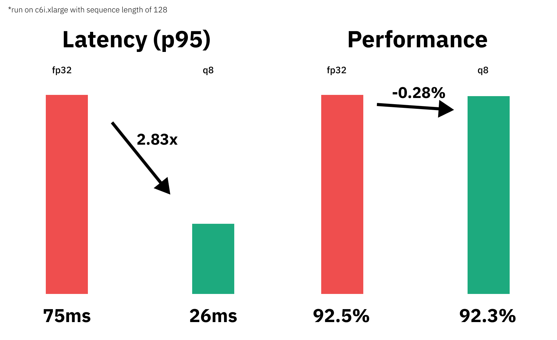
In our previous lesson's case study, we saw the results of quantizing a Wav2Vec 2.0 model. Let's revisit those results from the SpeechBrain tutorial. The original model had a certain WER and RTF, and after applying a hybrid static/dynamic quantization, the RTF improved significantly (faster inference) while the WER increased slightly (lower accuracy).
This image provides another excellent, concise example of this trade-off.
3. Case Studies: Analyzing Trade-offs Across Architectures
The effectiveness of a quantization strategy heavily depends on the model's architecture. Let's watch a segment from a PyTorch presentation that compares the results of quantization on several well-known models.
Deep Dive on PyTorch Quantization - Chris Gottbrath
This video from the official PyTorch channel provides benchmark numbers that directly illustrate the trade-offs for different models.
Watch the section from 39:27 to 42:34. Pay close attention to the table comparing FP32 and quantized performance for three models: ResNet-50 (a CNN): Note the excellent trade-off achieved with post-training quantization (PTQ). BERT (a Transformer): Observe that dynamic quantization yields a significant speedup with virtually no accuracy loss. This reinforces why dynamic PTQ is well-suited for Transformer-based models. MobileNetV2 (a lightweight CNN): The presenter notes that a more advanced technique (QAT) was needed to achieve good results. This sets the stage for our next topic.
These case studies highlight a crucial point: there is no one-size-fits-all solution. A strategy that works well for a large CNN might not be optimal for a Transformer or a highly optimized mobile architecture.
4. Managing the Trade-off: Quantization-Aware Training (QAT)
What do you do when the accuracy degradation from Post-Training Quantization (PTQ) is unacceptable for your application? You can employ a more powerful, albeit more complex, technique: Quantization-Aware Training (QAT).
In QAT, you don't just quantize a fully trained model. Instead, you fine-tune the model for a few epochs while simulating the effects of quantization during the forward and backward passes. This allows the model to learn to compensate for the quantization noise, often recovering most of the accuracy lost during PTQ.
The same PyTorch video provides a great explanation of QAT and a compelling analysis of its benefits.
Deep Dive on PyTorch Quantization - Chris Gottbrath
Let's continue with the PyTorch video to understand QAT and see a direct comparison of different quantization strategies.
First, watch from 34:03 to 39:27 to understand the concept of QAT. The key idea is fine-tuning the model with 'fake quantize' nodes to simulate quantization. \nNext, watch the ablation study for MobileNetV2 from 42:34 to 45:15. This is a critical comparison. Note how: Per-tensor PTQ results in a large accuracy drop (6%). Per-channel PTQ improves it, but the drop is still significant (5%). QAT recovers almost all the performance, with only a 0.4% drop.\nThis clearly demonstrates how choosing a more advanced technique can shift the trade-off in your favor.
5. Visualizing the Trade-off: Perceptual Quality and Pareto Fronts
For the ASR tasks we've discussed, WER is a good metric. But for your broader interests in TTS and generative audio, the trade-off is often measured in perceptual audio quality versus bit rate. A lower bit rate means more compression (more aggressive quantization) and a smaller file size, but it can introduce audible artifacts.
This next video intuitively demonstrates this concept using Residual Vector Quantization (RVQ), a technique used in modern neural audio codecs like EnCodec.
Residual Vector Quantization for Audio and Speech Embeddings
This video from the Efficient NLP channel provides a fantastic demonstration of the audio quality vs. bit rate trade-off.
Watch from 07:01 to 10:17. Focus on: The relationship between the number of quantization iterations (nq) and the final bit rate. The chart showing the quality score degrading as the bit rate drops below 6 kbps. The audio examples (which the speaker describes), where you can clearly 'hear' the artifacts at very low bit rates (1.5, 3 kbps), while the 6 kbps version sounds very close to the original.
A formal way to represent these trade-offs is by plotting a Pareto Front. In our context, a Pareto front shows the set of optimal models where you cannot improve one metric (e.g., reduce latency) without degrading another (e.g., increasing WER). The goal is to find models that lie on this "optimal" curve.
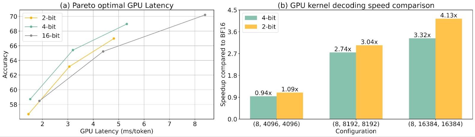
Looking at graph (a), you can see the trade-off clearly. For any given quantization strategy (e.g., 4-bit), to get higher accuracy (move right), you must accept higher latency (move up). The best strategies are those that push the curve "down and to the left," offering better accuracy for the same latency. Graph (b) quantifies the speed benefit, showing that 2-bit quantization can be over 4x faster than 16-bit.
Conclusion
In this lesson, you've learned to systematically evaluate the results of model quantization. This is a critical skill for any AI engineer, as deploying models in the real world is always a game of balancing constraints.
Key Takeaways:
- Quantization creates a three-way trade-off between model size, inference speed, and performance.
- This trade-off is rooted in the move to lower-precision data types (like INT8), which reduces memory and accelerates computation but introduces quantization error.
- The impact must be measured with concrete metrics relevant to the task (e.g., WER/RTF for ASR, bit rate/perceptual quality for audio codecs).
- The optimal balance depends on the model architecture and application requirements. Techniques like QAT and per-channel quantization provide powerful tools to manage this trade-off and recover performance.
- Visualizations like Pareto fronts are the standard way to represent and compare the efficiency of different optimization strategies.
Preview of the Next Lesson:
Now that you can train, optimize, and evaluate a speech model, the next step is to prepare it for deployment in different environments. In the next lesson, you will learn how to export a trained PyTorch speech model to ONNX format, a crucial step for creating framework-agnostic, high-performance inference applications.