Quantizing Speech Models: Dynamic and Static Approaches

Hello! Welcome to the second lesson in our module on model optimization.

In our previous lesson, we explored knowledge distillation, a powerful training-time technique for compressing large models. We saw how a smaller "student" model could learn from a larger "teacher," resulting in significant speed-ups with minimal accuracy loss, as demonstrated by Distil-Whisper.

Today, we shift our focus to post-training optimization. You'll learn about quantization, one of the most widely used techniques for reducing a model's memory footprint and accelerating its inference speed after it has already been trained. This lesson will cover the core mathematical principles of quantization and then guide you through applying the two main post-training approaches—dynamic and static quantization—to a speech model.

1. What is Quantization and Why Do We Need It?

At its core, quantization is the process of reducing the precision of the numbers used to represent a model's parameters (weights) and, in some cases, its activations. Typically, models are trained using 32-bit floating-point numbers (FP32). Quantization converts these FP32 values into lower-precision formats, most commonly 8-bit integers (INT8).

This seemingly simple conversion has profound benefits:

• Reduced Memory Footprint: An INT8 value uses only 1 byte of memory compared to 4 bytes for an FP32 value. This leads to a theoretical 4x reduction in model size.
• Faster Inference: Integer arithmetic operations are significantly faster than floating-point operations on most modern CPUs and specialized hardware.
• Lower Energy Consumption: Faster, simpler computations mean less power is used, which is critical for deployment on battery-powered devices like smartphones.

To get a clear overview of these concepts, let's start with a short video.

2. The Mathematics of Quantization

Quantization isn't just simple rounding. It's a mapping from a continuous range of high-precision floating-point values to a discrete set of lower-precision integer values. This mapping is defined by two key parameters: the scale factor (S) and the zero-point (Z).

The fundamental relationship is:

$$\text{real\_value}\approx S\times (\text{quantized\_value}-Z)$$

And the quantization process itself is the inverse:

$$\text{quantized\_value}=\text{round}\left(\frac{\text{real\_value}}{S}+Z\right)$$

• Scale (S): A positive floating-point number that defines the step size of the quantization. It determines the mapping between the original FP32 range and the target INT8 range.
• Zero-Point (Z): An integer that ensures the real value of 0.0 maps correctly to a quantized integer value. This is crucial for accurately representing padding, biases, and activations from functions like ReLU.

To dive deeper into the mathematics and see how S and Z are calculated, let's study a clear, concise guide.

There are two primary schemes for applying this mapping: asymmetric and symmetric.

• Asymmetric Quantization: This is the general approach described by the formula above. It can map any FP32 range [min, max] to the full INT8 range (e.g., [0, 255] for unsigned INT8 or [-128, 127] for signed INT8). The zero-point Z can be any value within the quantized range.
• Symmetric Quantization: This is a constrained version where the zero-point Z is fixed at 0. The FP32 range is assumed to be symmetric around zero, like [-max_abs, +max_abs]. This is often used for model weights, which tend to have a distribution centered around zero.

The following video provides a detailed walkthrough of both schemes, including the specific formulas for calculating S and Z in each case.

3. Post-Training Quantization (PTQ) Workflows

As the name suggests, Post-Training Quantization is applied to a model that has already been fully trained. This is highly convenient as it doesn't require retraining. There are two main PTQ workflows, which differ in how they handle model activations—the outputs of intermediate layers, which are data-dependent. Model weights are always known ahead of time and can be quantized offline in both cases.

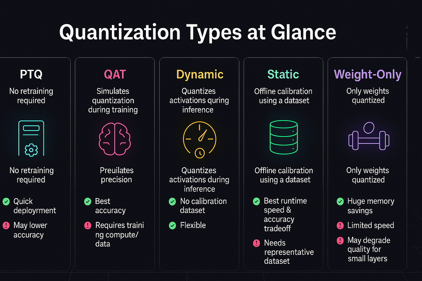
Let's read a quick comparison of these two approaches.

Now, let's explore each workflow in more detail.

3.1. Dynamic Quantization

In dynamic quantization, weights are quantized offline, but activations are quantized on-the-fly during inference. For each input that passes through a layer, the framework calculates the min/max range of the activation tensor and determines the appropriate scale and zero-point just-in-time.

• Pros: Very simple to apply, often just a one-line code change. No calibration data is needed. It's robust to varying distributions in activation values.
• Cons: The on-the-fly calculation of scale and zero-point adds computational overhead, which can sometimes limit the overall speed-up.
• Best for: Models where memory bandwidth is the bottleneck and activation distributions vary significantly, such as LSTMs and Transformers.

Applying dynamic quantization in PyTorch is straightforward. You call torch.quantization.quantize_dynamic, specifying the model and the layers to be quantized.

# Pseudocode for Dynamic Quantization
import torch.quantization




# Load your pre-trained FP32 model
model_fp32.eval() 




# Apply dynamic quantization
model_dynamic_quantized = torch.quantization.quantize_dynamic(
    model_fp32,  # the model to be quantized
    {torch.nn.Linear},  # set of layer types to quantize
    dtype=torch.qint8  # target data type
)




# The model is now ready for inference

3.2. Static Quantization

In static quantization, both weights and activations are quantized offline before inference. To determine the scale and zero-point for the activations, this method requires a calibration step.

Calibration Process:

1. Prepare: You insert "observer" modules into the model graph. These observers will watch the activation tensors that flow through the model.
2. Calibrate: You pass a small, representative set of data samples (e.g., 100-1000 audio clips) through the prepared model. The observers record the min and max values of the activations.
3. Convert: Using the statistics gathered by the observers, the framework calculates fixed scale and zero-point values for each activation tensor. The observers are removed, and the layers are permanently converted to their quantized versions.

• Pros: Potentially the fastest inference speed, as all quantization calculations are done offline.
• Cons: Requires a calibration step and a representative dataset. Performance can degrade if the calibration data doesn't reflect the distribution of real-world inference data.
• Best for: Models with predictable activation distributions, such as CNNs, where the calibration process can capture the typical data range effectively.

The following video provides an excellent, practical code walkthrough of the static quantization workflow in PyTorch.

4. Case Study: Quantizing a Wav2Vec 2.0 Model

Now let's apply this knowledge to a real-world speech recognition model. Your experience with ASR models makes this a perfect case study. We will follow a tutorial from SpeechBrain that quantizes a wav2vec 2.0 model.

A key challenge in quantizing complex models like this is that a single strategy (all-dynamic or all-static) might not be optimal. Instead, a hybrid approach is often best, where different parts of the model are quantized using different techniques.

The first step is to analyze the model architecture and decide on a quantization strategy.

After devising a strategy, we can implement it. The SpeechBrain tutorial provides a custom function that neatly wraps PyTorch's quantization API to apply this hybrid static-and-dynamic scheme. Let's look at the implementation and the results.

This case study perfectly illustrates that applying quantization in practice is not just about calling an API; it involves analyzing the model architecture, understanding the capabilities and limitations of the tools, and making informed decisions to balance performance and accuracy.

Conclusion

In this lesson, we have moved from the theory of quantization to its practical application. You've learned how to reduce a model's precision from FP32 to INT8 to gain significant improvements in size and speed.

Key Takeaways:

• Quantization is a post-training optimization technique that maps high-precision floating-point values to low-precision integers using a scale and zero-point.
• Dynamic PTQ is simple to implement and quantizes activations on-the-fly, making it suitable for models with variable activation ranges like Transformers.
• Static PTQ quantizes activations offline after a calibration step. It can offer better performance but requires a representative dataset and careful setup.
• Practical Application on complex models like wav2vec 2.0 often requires a hybrid strategy, applying different quantization methods to different parts of the model to achieve the best results.

Preview of the Next Lesson:

We've now seen the direct result of quantization on a speech model: a trade-off between inference speed (RTF) and accuracy (WER). In our next lesson, we will formalize this by learning how to evaluate the trade-off between model size, inference speed, and performance degradation after quantization. This will equip you to systematically measure and report the impact of your optimization efforts.