Multi-Query Attention: KV Cache Reduction

Introduction

In our last lesson, we successfully benchmarked FlashAttention and confirmed its effectiveness in optimizing the computation of attention by minimizing memory I/O between GPU SRAM and HBM. This was a crucial step in speeding up the forward pass.

However, a different and equally significant memory challenge arises during autoregressive inference: the KV cache. As we generate tokens one by one, we must store the Key (K) and Value (V) tensors for all previously generated tokens to maintain context. This cache grows linearly with the sequence length and can consume enormous amounts of VRAM, often becoming the primary memory bottleneck for long-context generation. FlashAttention optimizes the calculation but does not reduce the size of the data that must be stored.

Today, we address this second bottleneck. Your learning outcome is to implement Multi-Query Attention (MQA) and measure the reduction in KV cache size compared to standard Multi-Head Attention (MHA). We will explore the architectural change behind MQA, implement it in PyTorch, and precisely calculate the VRAM savings it provides.

From Multi-Head to Multi-Query Attention

Before we dive into code, let's establish a strong conceptual model of MHA and MQA. Standard Multi-Head Attention (MHA) uses independent Key and Value projection heads for each Query head. This allows each head to learn different relational patterns but comes at a high memory cost for the KV cache. Multi-Query Attention (MQA) proposes a simple but powerful change: all Query heads share a single Key and Value head.

To get a clear overview of the problem and the MQA solution, let's watch a segment from a talk by Julien Simon.

The key insight is the change in the number of K and V heads.

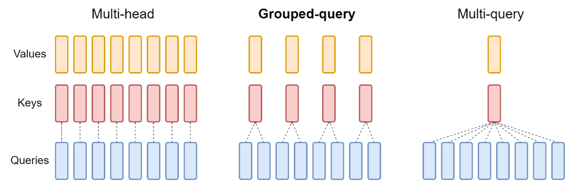
This simple change has profound implications for the KV cache. Let's dig into the numbers.

Calculating KV Cache Memory

The size of the KV cache is a direct function of the model's architecture and the generation parameters. The article KV Cache Memory: Calculating GPU Requirements for LLM... provides a clear derivation of the formula we need.

As you've read, the total memory for the KV cache is:
$\text{KV Cache Memory}=2\times L\times B\times T\times H_{kv}\times D_h\times \text{bytes\_per\_element}$
where:

• 2: For storing both K and V tensors.
• L: Number of transformer layers.
• B: Batch size.
• T: Sequence length (number of tokens in the cache).
• $H_{kv}$: Number of Key-Value heads.
• $D_h$: Dimension of each head.

The crucial difference lies in $H_{kv}$:

• For MHA: The number of KV heads is equal to the number of query heads ($H_q$). So, $H_{kv}=H_q$.
• For MQA: There is only one KV head shared by all query heads. So, $H_{kv}=1$.

This means MQA reduces the KV cache size by a factor of $H_q$. For a model with 32 attention heads, this is a 32x reduction in the memory required for the KV cache, a massive saving.

Practical Implementation and Measurement

Now, let's translate this into code. We will implement simplified MHA and MQA attention modules in PyTorch to demonstrate the difference in their structure and then use the formula to calculate the resulting KV cache size.

Create a new Python script and add the following code:

import torch
import torch.nn as nn




# --- Model Hyperparameters ---
# Let's use parameters similar to a Llama-like 7B model
D_MODEL = 4096  # Hidden dimension
NUM_HEADS = 32  # Number of query heads
HEAD_DIM = D_MODEL // NUM_HEADS  # 128




# --- 1. Multi-Head Attention (MHA) Implementation ---
class MHA(nn.Module):
    def __init__(self, d_model, num_heads):
        super().__init__()
        self.d_model = d_model
        self.num_heads = num_heads
        self.head_dim = d_model // num_heads




        # In MHA, K and V projections have the same dimension as Q
        self.q_proj = nn.Linear(d_model, d_model)
        self.k_proj = nn.Linear(d_model, d_model) # Projects to num_heads * head_dim
        self.v_proj = nn.Linear(d_model, d_model) # Projects to num_heads * head_dim
        self.out_proj = nn.Linear(d_model, d_model)

    def forward(self, x):
        batch_size, seq_len, _ = x.shape
        



        # Project and reshape
        q = self.q_proj(x).view(batch_size, seq_len, self.num_heads, self.head_dim).transpose(1, 2)
        k = self.k_proj(x).view(batch_size, seq_len, self.num_heads, self.head_dim).transpose(1, 2)
        v = self.v_proj(x).view(batch_size, seq_len, self.num_heads, self.head_dim).transpose(1, 2)
        



        # For this exercise, we only care about the shape of K and V
        return k, v




# --- 2. Multi-Query Attention (MQA) Implementation ---
class MQA(nn.Module):
    def __init__(self, d_model, num_heads):
        super().__init__()
        self.d_model = d_model
        self.num_heads = num_heads
        self.head_dim = d_model // num_heads




        # Q projection is the same as MHA
        self.q_proj = nn.Linear(d_model, d_model)
        



        # In MQA, K and V projections are for a SINGLE head
        self.k_proj = nn.Linear(d_model, self.head_dim) # Projects to just head_dim
        self.v_proj = nn.Linear(d_model, self.head_dim) # Projects to just head_dim
        
        self.out_proj = nn.Linear(d_model, d_model)

    def forward(self, x):
        batch_size, seq_len, _ = x.shape
        



        # Project and reshape
        q = self.q_proj(x).view(batch_size, seq_len, self.num_heads, self.head_dim).transpose(1, 2)
        



        # K and V have a different shape now
        k = self.k_proj(x).view(batch_size, seq_len, 1, self.head_dim).transpose(1, 2)
        v = self.v_proj(x).view(batch_size, seq_len, 1, self.head_dim).transpose(1, 2)
        
        return k, v




# --- 3. Verify the shapes ---
mha_layer = MHA(D_MODEL, NUM_HEADS)
mqa_layer = MQA(D_MODEL, NUM_HEADS)

dummy_input = torch.randn(1, 1024, D_MODEL) # (batch, seq_len, d_model)

k_mha, v_mha = mha_layer(dummy_input)
k_mqa, v_mqa = mqa_layer(dummy_input)

print(f"--- Shape Verification ---")
print(f"MHA Key Shape: {k_mha.shape}") # Expected: [1, 32, 1024, 128]
print(f"MQA Key Shape: {k_mqa.shape}") # Expected: [1, 1, 1024, 128]
print("-" * 25)

The most important lines are the definitions of k_proj and v_proj. In MHA, they project to the full d_model dimension, which is then split among 32 heads. In MQA, they project directly to a single head_dim, creating only one head for K and V. The print statements confirm that the number of heads for K and V (dim=1) is 32 for MHA and 1 for MQA.

Exercise: Quantify the KV Cache Reduction

Now, let's use the formula to calculate the VRAM required for the full KV cache of a model and see the impact of MQA. Add the following function and calculations to your script.

# --- 4. KV Cache Calculation Function ---
def calculate_kv_cache_memory(num_layers, batch_size, seq_len, num_kv_heads, head_dim, dtype_bytes=2):
    """Calculates the memory required for the KV cache in GB."""
    



    # Formula: 2 * L * B * T * H_kv * D_h * bytes
    total_elements = 2 * num_layers * batch_size * seq_len * num_kv_heads * head_dim
    memory_bytes = total_elements * dtype_bytes
    memory_gb = memory_bytes / (1024**3)
    
    return memory_gb




# --- 5. Run the Calculation ---
# Realistic model and inference parameters
NUM_LAYERS = 32
BATCH_SIZE = 1
SEQ_LEN = 4096
DTYPE_BYTES = 2 # for float16/bfloat16




# Calculate for MHA
num_kv_heads_mha = NUM_HEADS
kv_cache_mha_gb = calculate_kv_cache_memory(
    num_layers=NUM_LAYERS,
    batch_size=BATCH_SIZE,
    seq_len=SEQ_LEN,
    num_kv_heads=num_kv_heads_mha,
    head_dim=HEAD_DIM,
    dtype_bytes=DTYPE_BYTES
)




# Calculate for MQA
num_kv_heads_mqa = 1
kv_cache_mqa_gb = calculate_kv_cache_memory(
    num_layers=NUM_LAYERS,
    batch_size=BATCH_SIZE,
    seq_len=SEQ_LEN,
    num_kv_heads=num_kv_heads_mqa,
    head_dim=HEAD_DIM,
    dtype_bytes=DTYPE_BYTES
)

reduction_factor = kv_cache_mha_gb / kv_cache_mqa_gb

print(f"\n--- KV Cache Memory Calculation ---")
print(f"Model: {NUM_LAYERS} layers, {NUM_HEADS} heads, head_dim {HEAD_DIM}")
print(f"Inference: batch={BATCH_SIZE}, seq_len={SEQ_LEN}, dtype=fp16\n")

print(f"MHA KV Cache Size: {kv_cache_mha_gb:.2f} GB")
print(f"MQA KV Cache Size: {kv_cache_mqa_gb:.2f} GB")
print(f"\nMemory Reduction Factor: {reduction_factor:.0f}x")

When you run this script, you will see the output confirming a 32x reduction in KV cache memory. For a 7B model with a 4K context, MHA requires 2 GB for the cache, whereas MQA requires only 64 MB. This difference is critical; it can determine whether a model fits on a given GPU, especially when serving multiple users (increasing the batch size) or handling very long contexts.

Conclusion

In this lesson, you have moved from optimizing attention computation to optimizing attention memory. You have seen how a targeted architectural change—sharing Key and Value heads—can lead to dramatic system-level improvements.

Key Takeaways:

• Multi-Query Attention (MQA) reduces the memory footprint of the KV cache by having all query heads share a single key and value head.
• The memory reduction is directly proportional to the number of query heads ($H_q$). For a model with 32 heads, MQA offers a 32x reduction in KV cache size compared to MHA.
• This saving is critical for enabling long-context inference and high-throughput serving on memory-constrained hardware.
• The trade-off is a potential minor decrease in model quality for a significant gain in inference efficiency—a classic systems engineering decision.

Preview of the Next Lesson:

MQA represents one extreme (a single KV head), while MHA represents the other (one KV head per query head). What if there's a middle ground? In our next lesson, we will generalize this concept to Grouped-Query Attention (GQA). You will implement GQA and analyze how it allows you to balance the trade-off between memory footprint and model quality, giving you a tunable parameter for performance engineering.