FlashAttention Benchmarking

Introduction

In our previous lesson, we dissected the theory behind FlashAttention, exploring how its IO-aware design, combining tiling and an online softmax algorithm, avoids the massive O(N^2) memory-I/O bottleneck of standard attention. We concluded that by keeping intermediate computations in fast SRAM, FlashAttention should be significantly faster and more memory-efficient, especially for long sequences.

Today, we move from theory to practice. Your learning outcome is to benchmark standard attention vs. a FlashAttention implementation, measuring speedup and memory savings across varying sequence lengths. This is a purely practical lesson where you will write code to generate empirical data, directly testing the claims from the last session. By the end, you'll have firsthand, quantitative proof of FlashAttention's impact and a robust methodology for benchmarking GPU operations.

The Experimental Setup: Code and Methodology

To conduct a fair benchmark, we need three components:

1. A baseline standard attention implementation that reflects the memory-inefficient approach.
2. An optimized FlashAttention implementation to compare against.
3. A benchmarking harness that accurately measures latency and peak memory usage on the GPU.

The following article provides an excellent foundation for our experiment. It walks through setting up a benchmark comparing a naive attention implementation with PyTorch's native FlashAttention.

Step 1: Implementing the Benchmarking Harness

We will write a Python script to perform this benchmark. Let's start by setting up the environment and the core benchmarking function. We'll adapt the bench_attention function from the article to measure not only latency but also peak memory consumption, which is crucial for our analysis. We can achieve this using torch.cuda.max_memory_allocated().

Here is the complete setup code. Create a new Python file and add the following:

import torch
import torch.nn.functional as F
import numpy as np
import time
from tqdm import tqdm
import matplotlib.pyplot as plt




# Check for CUDA availability
if not torch.cuda.is_available():
    print("CUDA is not available. This benchmark requires a GPU.")
    exit()

device = torch.device("cuda")




# --- 1. Standard Attention (Naive Implementation) ---
# This is our baseline, mirroring the memory-inefficient approach.
def standard_scaled_dot_product_attention(query, key, value, is_causal=False):
    """
    Computes scaled dot product attention in eager mode, materializing the large attention matrix.
    """



    # N = seq_len, d = head_dim
    # query, key, value: (batch_size, num_heads, N, d)
    
    scale_factor = 1 / np.sqrt(query.size(-1))
    



    # S = QK^T -> (batch_size, num_heads, N, N)
    # This materializes the N x N matrix in memory (HBM)
    attn_weight = (query @ key.transpose(-2, -1)) * scale_factor

    if is_causal:
        seq_len = query.size(-2)
        causal_mask = torch.triu(torch.ones(seq_len, seq_len, device=device, dtype=torch.bool), diagonal=1)
        attn_weight = attn_weight.masked_fill(causal_mask, -torch.inf)




    # P = softmax(S) -> (batch_size, num_heads, N, N)
    # This is also stored in HBM
    attn_weight = torch.softmax(attn_weight, dim=-1)
    



    # O = PV -> (batch_size, num_heads, N, d)
    return attn_weight @ value


```grasp
{
  "type": "exercise",
  "id": "67c81172-ca7b-4d5c-968c-37e13f09f1e6"
}

--- 2. The Benchmarking Function ---

This harness measures both latency and peak memory.

def benchmark_attention(seq_len, attention_fn, num_repeats=100, batch_size=1, num_heads=32, embed_dim=128, dtype=torch.float16):
"""
Measures average latency and peak memory for an attention function.
"""
query = torch.randn(batch_size, num_heads, seq_len, embed_dim, device=device, dtype=dtype)
key = torch.randn(batch_size, num_heads, seq_len, embed_dim, device=device, dtype=dtype)
value = torch.randn(batch_size, num_heads, seq_len, embed_dim, device=device, dtype=dtype)

# Warmup
for _ in range(10):
    _ = attention_fn(query, key, value, is_causal=True)
torch.cuda.synchronize()




# Measure Latency
start_event = torch.cuda.Event(enable_timing=True)
end_event = torch.cuda.Event(enable_timing=True)

start_event.record()
for _ in range(num_repeats):
    _ = attention_fn(query, key, value, is_causal=True)
end_event.record()
torch.cuda.synchronize()
latency_ms = start_event.elapsed_time(end_event) / num_repeats




# Measure Memory
torch.cuda.reset_peak_memory_stats()
_ = attention_fn(query, key, value, is_causal=True)
torch.cuda.synchronize()
peak_memory_mb = torch.cuda.max_memory_allocated() / (1024 ** 2)

return latency_ms, peak_memory_mb

Notice the key components:
-   Our `standard_scaled_dot_product_attention` explicitly performs the matrix multiplication (`@`), materializing the `(N, N)` attention score matrix. This is the HBM-intensive operation we want to profile.
-   The `benchmark_attention` function uses CUDA events for precise timing and `reset_peak_memory_stats` to isolate the memory usage of a single forward pass.




### Step 2: Running the Experiment

Now, let's use our harness to collect data. We will loop through a range of sequence lengths and run the benchmark for both standard attention and FlashAttention. In modern PyTorch, FlashAttention is the default backend for `F.scaled_dot_product_attention` when the inputs are appropriate (on CUDA, fp16/bf16, and causal).

Add the following code to your script to execute the experiment:

```python



# --- 3. Run the Benchmark ---
sequence_lengths = np.arange(512, 8192 + 1, 512)




# Data storage
results = {
    "standard": {"latencies": [], "memories": []},
    "flash": {"latencies": [], "memories": []}
}

print("Running benchmark...")
for seq_len in tqdm(sequence_lengths):



    # Benchmark standard attention
    std_latency, std_memory = benchmark_attention(
        seq_len, 
        standard_scaled_dot_product_attention
    )
    results["standard"]["latencies"].append(std_latency)
    results["standard"]["memories"].append(std_memory)
    



    # Benchmark PyTorch's optimized attention (which will use FlashAttention)
    flash_latency, flash_memory = benchmark_attention(
        seq_len,
        F.scaled_dot_product_attention
    )
    results["flash"]["latencies"].append(flash_latency)
    results["flash"]["memories"].append(flash_memory)

print("Benchmark complete.")

Step 3: Analyzing the Results

The final step is to visualize and interpret the data. We expect to see FlashAttention's latency scale better than standard attention's, and its memory usage remain low and scale linearly, while standard attention's memory usage scales quadratically.

Add this plotting code to your script:

# --- 4. Plot the Results ---
fig, axs = plt.subplots(1, 3, figsize=(20, 5))




# Plot 1: Latency
axs[0].plot(sequence_lengths, results["standard"]["latencies"], label="Standard Attention", marker='o')
axs[0].plot(sequence_lengths, results["flash"]["latencies"], label="FlashAttention", marker='o')
axs[0].set_xlabel("Sequence Length")
axs[0].set_ylabel("Latency (ms)")
axs[0].set_title("Latency vs. Sequence Length")
axs[0].legend()
axs[0].grid(True)




# Plot 2: Peak Memory
axs[1].plot(sequence_lengths, results["standard"]["memories"], label="Standard Attention", marker='o')
axs[1].plot(sequence_lengths, results["flash"]["memories"], label="FlashAttention", marker='o')
axs[1].set_xlabel("Sequence Length")
axs[1].set_ylabel("Peak Memory (MB)")
axs[1].set_title("Peak Memory vs. Sequence Length")
axs[1].legend()
axs[1].grid(True)




# Plot 3: Speedup
speedup = [s / f for s, f in zip(results["standard"]["latencies"], results["flash"]["latencies"])]
axs[2].plot(sequence_lengths, speedup, label="Speedup", marker='o', color='green')
axs[2].set_xlabel("Sequence Length")
axs[2].set_ylabel("Speedup (Standard / Flash)")
axs[2].set_title("Speedup vs. Sequence Length")
axs[2].legend()
axs[2].grid(True)

plt.tight_layout()
plt.show()

When you run the full script, you should see plots that look conceptually similar to these benchmark results from the FlashAttention paper and other analyses.

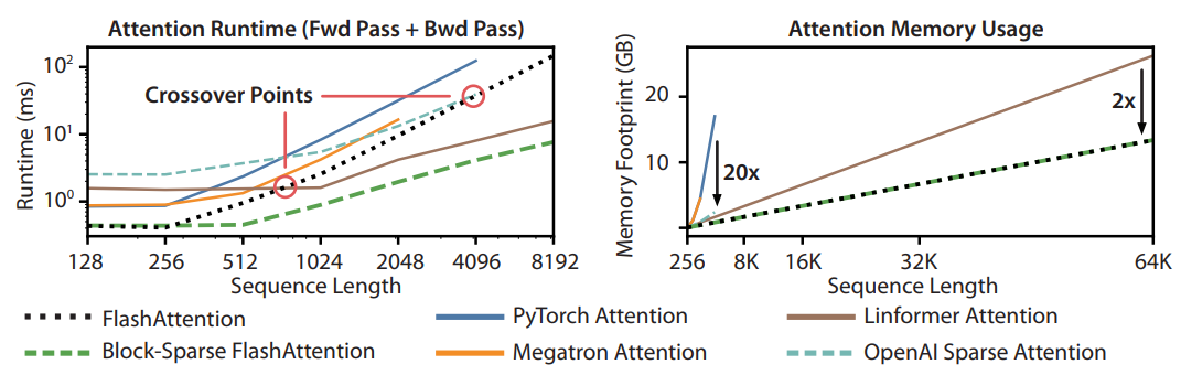
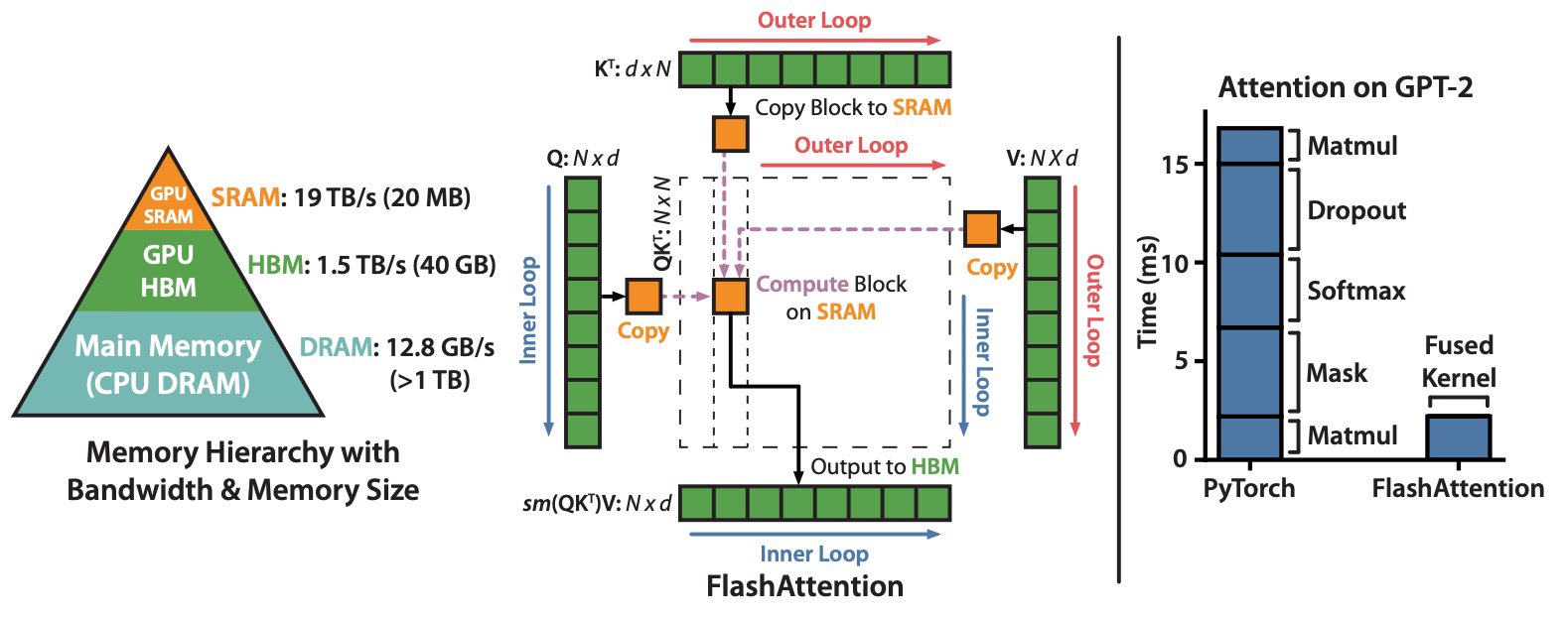
Your own plots will provide concrete, empirical validation of the theoretical benefits we discussed. You should observe:

1. Latency: The gap between standard and FlashAttention's latency will widen as the sequence length increases.
2. Memory: Standard attention's memory will grow quadratically (O(N^2)), likely causing an out-of-memory error on your GPU at longer sequence lengths. FlashAttention's memory will grow linearly (O(N)), remaining manageable.
3. Speedup: The speedup factor will not be constant; it will increase with the sequence length, as the O(N^2) cost of the naive method becomes more dominant.

This experiment provides a powerful and practical confirmation of how algorithmic choices, when co-designed with hardware characteristics, lead to dramatic performance improvements in real-world systems.

Conclusion

In this lesson, you stepped into the role of a systems performance engineer. You formulated a hypothesis based on theory, designed and implemented a rigorous benchmark, and analyzed the resulting data to draw a quantitative conclusion.

Key Takeaways:

• Empirical Validation: We have now proven with hard data that FlashAttention delivers on its promises, offering significant speedups (especially at long sequence lengths) and drastically reducing peak memory consumption.
• Quadratic vs. Linear Scaling: You observed the practical consequences of O(N^2) memory complexity in standard attention, which quickly becomes untenable, versus the manageable O(N) complexity of FlashAttention.
• Benchmarking as a Tool: You now have a reusable code template for micro-benchmarking GPU operations, measuring both latency with CUDA events and peak memory usage with PyTorch utilities.

Preview of the Next Lesson:

FlashAttention masterfully optimizes the computation of the attention scores. However, it does not address a different, major memory bottleneck in autoregressive decoding: the KV Cache. As we generate tokens one by one, the size of the stored keys and values grows linearly with the sequence length, consuming a vast amount of VRAM. In our next lesson, we will tackle this problem by implementing Multi-Query Attention (MQA) and measuring its direct impact on reducing the KV cache size.