From MQA to GQA: A Trade-off Analysis

Introduction

In our last lesson, we explored Multi-Query Attention (MQA) as a powerful technique to drastically reduce the memory footprint of the KV cache. We saw that by sharing a single Key and Value head across all Query heads, MQA offers a massive reduction in memory, but this comes at the potential cost of model quality. MHA and MQA represent two extremes on the spectrum of attention design: maximum expressiveness vs. maximum memory efficiency.

This raises a natural question for a systems engineer: can we control this trade-off? The answer is yes, and that brings us to today's topic. Your learning outcome for this lesson is to generalize the MQA implementation to Grouped-Query Attention (GQA) and analyze its trade-off between memory footprint and model quality.

GQA provides a tunable "knob" between MHA and MQA, allowing you to choose a balance that fits your specific hardware constraints and performance requirements. We will implement it, measure its impact on memory, and analyze performance data to understand why it has become the de-facto standard for modern high-performance LLMs.

From Extremes to a Middle Ground: Understanding GQA

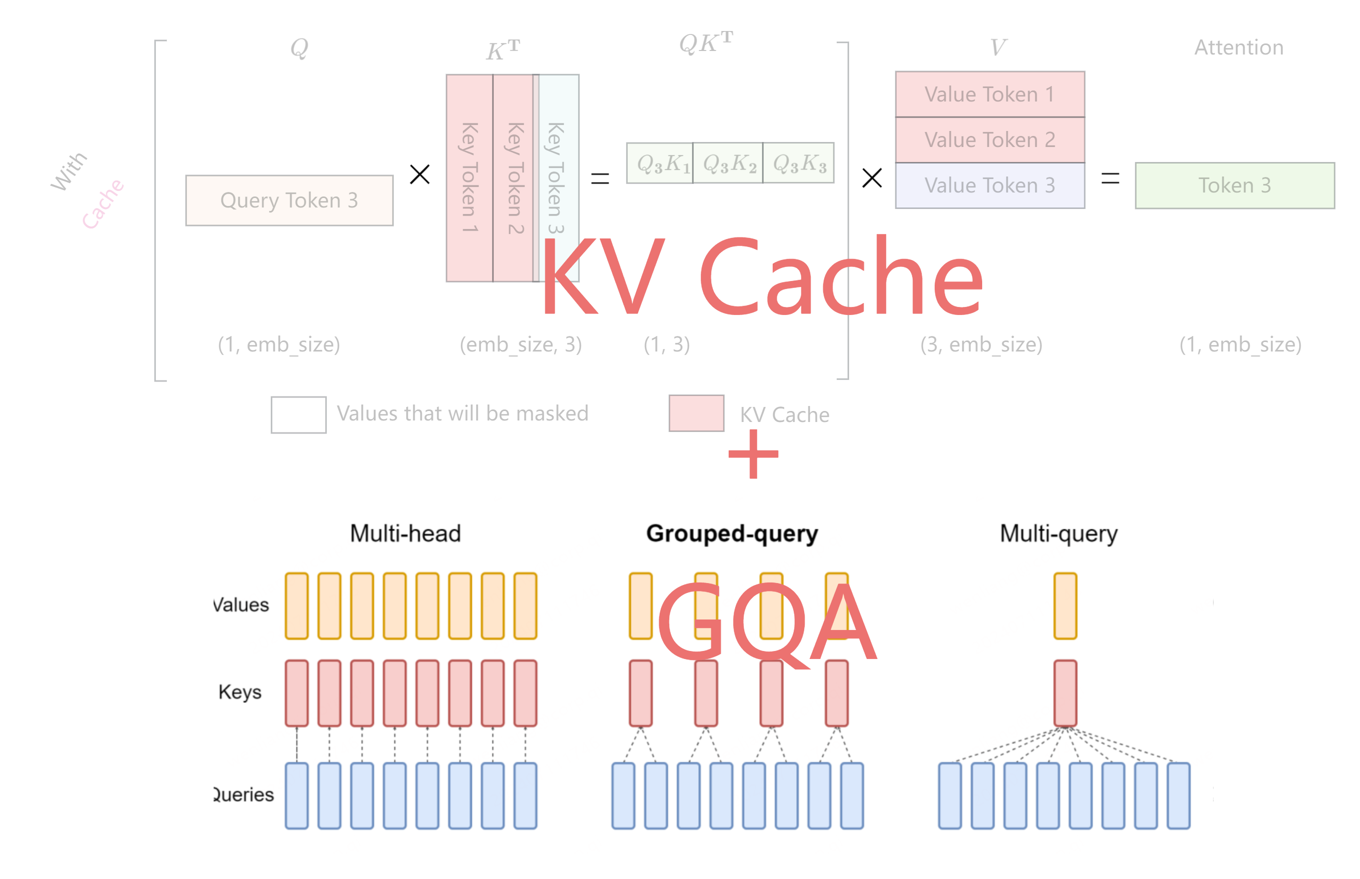
Grouped-Query Attention works by dividing the total number of query heads into several smaller groups. Within each group, all query heads share a single key and value head.

• If you have as many groups as you have query heads, each group contains one query head, and you recover Multi-Head Attention (MHA).
• If you have only one group, all query heads share a single KV head, and you recover Multi-Query Attention (MQA).

This elegant generalization allows us to explore the space between these two extremes. To get a clear visual and conceptual overview, let's watch a short, excellent explanation.

The video makes the relationship clear. GQA isn't a completely new architecture, but rather a generalization that unifies MHA and MQA.

Let's solidify this understanding by looking at a more formal definition.

With this conceptual foundation, we can now move to the practical implementation.

Hands-on: Generalizing MQA to GQA

We will now modify the MQA implementation from the previous lesson to create a more general GQA module. The key insight is that while the K and V projection layers will produce a smaller number of heads, we need to "broadcast" or "repeat" these heads to match the number of query heads before performing the attention score calculation. This is precisely the approach used in models like Llama 3.

The article "Understanding Grouped-Query Attention" provides a very clear PyTorch implementation that we can adapt.

Now, create a new Python script. We will build a single, flexible Attention class that can function as MHA, MQA, or GQA based on its configuration.

import torch
import torch.nn as nn




# --- Model & Attention Hyperparameters ---
D_MODEL = 4096
NUM_QUERY_HEADS = 32



# Let's use 8 KV heads, a common choice for GQA (e.g., Llama 2/3)
NUM_KV_HEADS = 8
HEAD_DIM = D_MODEL // NUM_QUERY_HEADS  # 128

class GroupedQueryAttention(nn.Module):
    def __init__(self, d_model, num_query_heads, num_kv_heads):
        super().__init__()



        # Assert that the heads configuration is valid
        assert d_model % num_query_heads == 0, "d_model must be divisible by num_query_heads"
        assert num_query_heads % num_kv_heads == 0, "num_query_heads must be divisible by num_kv_heads"
        
        self.d_model = d_model
        self.num_query_heads = num_query_heads
        self.num_kv_heads = num_kv_heads
        self.num_queries_per_kv = num_query_heads // num_kv_heads
        self.head_dim = d_model // num_query_heads
        



        # Projection layers
        self.q_proj = nn.Linear(d_model, d_model) # Projects to num_query_heads * head_dim
        self.k_proj = nn.Linear(d_model, num_kv_heads * self.head_dim) # Projects to a smaller dimension
        self.v_proj = nn.Linear(d_model, num_kv_heads * self.head_dim) # Projects to a smaller dimension
        
        self.out_proj = nn.Linear(d_model, d_model)

    def forward(self, x):
        batch_size, seq_len, _ = x.shape
        



        # --- Projections ---
        q = self.q_proj(x)
        k = self.k_proj(x)
        v = self.v_proj(x)
        



        # --- Reshape for multi-head processing ---
        q = q.view(batch_size, seq_len, self.num_query_heads, self.head_dim).transpose(1, 2)



        # K and V have fewer heads
        k = k.view(batch_size, seq_len, self.num_kv_heads, self.head_dim).transpose(1, 2)
        v = v.view(batch_size, seq_len, self.num_kv_heads, self.head_dim).transpose(1, 2)
        



        # --- Key Step: Repeat K and V heads to match Q heads ---
        # This is the "grouping" mechanism. Each KV head is duplicated to serve
        # a group of query heads.
        if self.num_queries_per_kv > 1:
            k = k.repeat_interleave(self.num_queries_per_kv, dim=1)
            v = v.repeat_interleave(self.num_queries_per_kv, dim=1)
        



        # The rest of the attention calculation is identical to MHA
        # We'll just return the K, V tensors for shape verification
        return k, v




# --- Verify the shapes for MHA, GQA, and MQA ---
dummy_input = torch.randn(1, 1024, D_MODEL) # (batch, seq_len, d_model)




# 1. MHA equivalent: num_kv_heads = num_query_heads
mha_layer = GroupedQueryAttention(D_MODEL, NUM_QUERY_HEADS, NUM_QUERY_HEADS)
k_mha, _ = mha_layer(dummy_input)




# 2. GQA: num_kv_heads is between 1 and num_query_heads
gqa_layer = GroupedQueryAttention(D_MODEL, NUM_QUERY_HEADS, NUM_KV_HEADS)
k_gqa, _ = gqa_layer(dummy_input)




# 3. MQA equivalent: num_kv_heads = 1
mqa_layer = GroupedQueryAttention(D_MODEL, NUM_QUERY_HEADS, 1)
k_mqa, _ = mqa_layer(dummy_input)

print(f"--- Shape Verification (Query Heads: {NUM_QUERY_HEADS}) ---")
print(f"MHA Key Shape (KV Heads={NUM_QUERY_HEADS}): {k_mha.shape}") # Expected: [1, 32, 1024, 128]
print(f"GQA Key Shape (KV Heads={NUM_KV_HEADS}):  {k_gqa.shape}") # Expected: [1, 32, 1024, 128]
print(f"MQA Key Shape (KV Heads=1):   {k_mqa.shape}") # Expected: [1, 32, 1024, 128]
print("\nNotice the shapes after `repeat_interleave` are identical.")
print("The difference lies in the underlying K,V projection and cache size.")

Run this script. The output confirms that after the repeat_interleave step, the K and V tensors have the same shape as the Q tensor, ready for the dot-product attention calculation. The magic happens before this step, in the smaller projection layers and, consequently, the smaller KV cache.

Exercise: Analyzing the Memory Trade-off

Let's now quantify the memory savings. We will reuse the calculate_kv_cache_memory function from the previous lesson and apply it to all three configurations. Add the following code to your script:

# --- KV Cache Calculation ---
def calculate_kv_cache_memory(num_layers, batch_size, seq_len, num_kv_heads, head_dim, dtype_bytes=2):
    """Calculates the memory required for the KV cache in GB."""
    total_elements = 2 * num_layers * batch_size * seq_len * num_kv_heads * head_dim
    memory_bytes = total_elements * dtype_bytes
    memory_gb = memory_bytes / (1024**3)
    return memory_gb




# Model and inference parameters
NUM_LAYERS = 32
BATCH_SIZE = 1
SEQ_LEN = 8192
DTYPE_BYTES = 2 # for float16/bfloat16




# Calculate for MHA
kv_cache_mha_gb = calculate_kv_cache_memory(
    NUM_LAYERS, BATCH_SIZE, SEQ_LEN, NUM_QUERY_HEADS, HEAD_DIM, DTYPE_BYTES
)




# Calculate for GQA
kv_cache_gqa_gb = calculate_kv_cache_memory(
    NUM_LAYERS, BATCH_SIZE, SEQ_LEN, NUM_KV_HEADS, HEAD_DIM, DTYPE_BYTES
)




# Calculate for MQA
kv_cache_mqa_gb = calculate_kv_cache_memory(
    NUM_LAYERS, BATCH_SIZE, SEQ_LEN, 1, HEAD_DIM, DTYPE_BYTES
)

print(f"\n--- KV Cache Memory Analysis ---")
print(f"Model: {NUM_LAYERS} layers, {NUM_QUERY_HEADS} Q-heads, head_dim {HEAD_DIM}")
print(f"Inference: batch={BATCH_SIZE}, seq_len={SEQ_LEN}, dtype=fp16\n")

print(f"MHA ({NUM_QUERY_HEADS} KV heads) Cache Size: {kv_cache_mha_gb:.2f} GB")
print(f"GQA ({NUM_KV_HEADS} KV heads) Cache Size:  {kv_cache_gqa_gb:.2f} GB")
print(f"MQA (1 KV head) Cache Size:     {kv_cache_mqa_gb:.2f} GB\n")

print(f"GQA reduces KV cache by a factor of {kv_cache_mha_gb / kv_cache_gqa_gb:.0f}x compared to MHA.")
print(f"MQA reduces KV cache by a factor of {kv_cache_mha_gb / kv_cache_mqa_gb:.0f}x compared to MHA.")

The output clearly demonstrates how GQA sits in the middle. For an 8K context length, a 7B-scale model requires over 4 GB for the MHA KV cache, which can be prohibitive. GQA reduces this to just over 1 GB, while MQA brings it down to ~130 MB. This 1 GB footprint is often a sweet spot for many consumer and data center GPUs, explaining GQA's popularity.

Analyzing the Performance vs. Quality Trade-off

We've established GQA's position in terms of memory. But what about model quality and speed? Evaluating quality requires extensive benchmarking, but we can analyze published results to understand the trade-off.

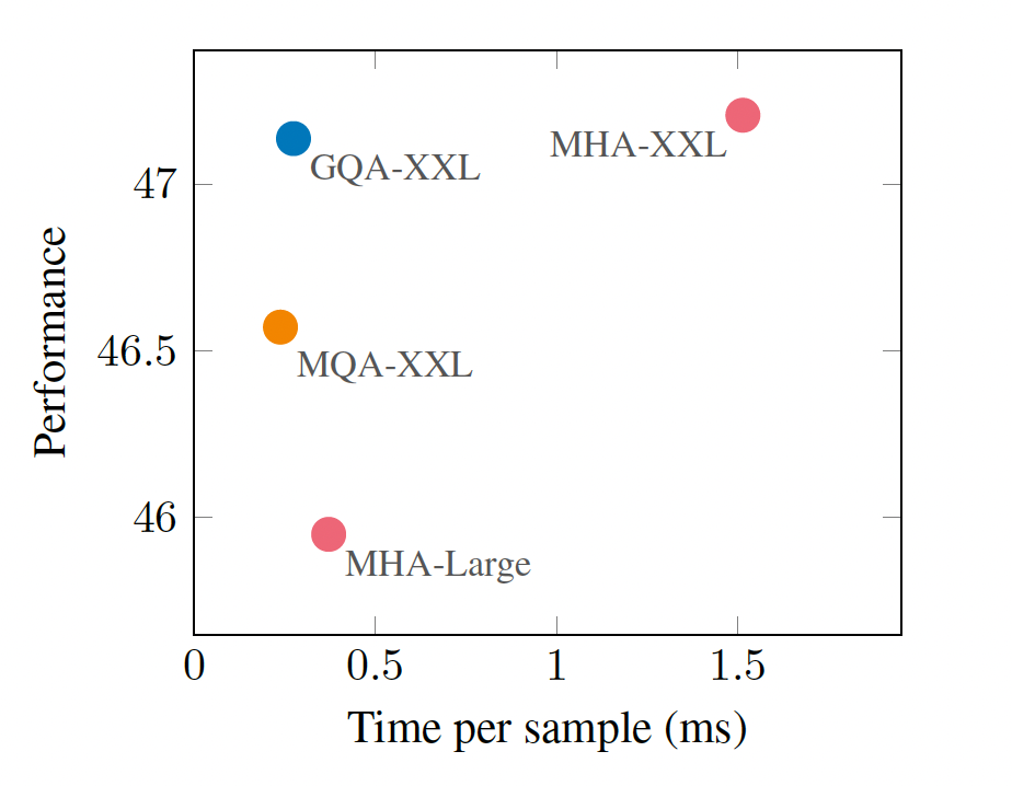
The chart above tells a compelling story. MHA is the best performing but the slowest. MQA is the fastest but has a noticeable performance drop. GQA manages to capture the best of both worlds: it achieves a speed-up very close to MQA while maintaining a performance level that is almost indistinguishable from MHA.

The comprehensive article Attention Mechanisms in Transformers also includes benchmark results comparing latency and memory for a Llama3 8B configuration.

These results confirm that GQA is not just a theoretical compromise but a highly practical one. It delivers most of the speed and memory benefits of MQA with a negligible impact on model quality, making it a superior choice for deploying high-performance LLMs.

Conclusion

In this lesson, you have generalized your understanding of attention mechanisms from the MHA/MQA extremes to the flexible GQA framework. You now have a clear mental model and the practical implementation knowledge of how modern LLMs balance performance and memory.

Key Takeaways:

• Grouped-Query Attention (GQA) is a generalization of MHA and MQA where the number of key-value heads (num_kv_heads) is a tunable hyperparameter.
• GQA behaves like MHA when num_kv_heads == num_query_heads and like MQA when num_kv_heads == 1.
• The implementation involves projecting K and V to a smaller dimension and then using torch.repeat_interleave to match the number of query heads.
• GQA provides a "sweet spot" in system design, achieving inference speed and memory usage close to the highly efficient MQA, while maintaining model quality nearly on par with the expensive MHA.

Preview of the Next Lesson:

So far, we have focused on the structure of the K and V tensors. In the next lesson, we will shift our focus to the runtime management of these tensors. You will implement a basic KV cache for autoregressive decoding and measure its memory growth over the generation sequence. This is the foundational component that enables efficient token-by-token generation and is the next logical step in building our request-to-token mental model.