RC Circuit Step Response: First-Order ODE

Hello! Welcome back to our course on Radioelectronics.

In our last session, we developed a strong conceptual understanding of transient and steady-state responses in first-order circuits. We saw how a capacitor's voltage changes over time and even used a "shortcut" formula to describe this behavior. Now, it's time to build that formula from the ground up.

Introduction

Approximate time to complete: 30-45 minutes.

Today's lesson focuses on a single, crucial learning outcome: Deriving the First-Order Ordinary Differential Equation (ODE) for an RC Circuit with a Step Input.

We will translate a physical circuit diagram into a mathematical equation using fundamental circuit laws. This process is at the heart of engineering analysis, bridging the gap between a physical system and its mathematical model. For someone with your background in both radiophysics and software development, this is like defining the core logic that governs a system's state transitions over time.

This lesson will focus exclusively on deriving the ODE. In our next lesson, we will tackle the methods for solving it.

1. The Building Blocks: Assembling Our Tools

To derive the governing equation for an RC circuit, we only need three fundamental principles, which should be familiar to you:

Kirchhoff's Voltage Law (KVL): The sum of the voltage drops around any closed loop in a circuit must equal the sum of the voltage sources in that loop.
Ohm's Law: The voltage across a resistor is proportional to the current flowing through it ( $v = i R$ ).
Capacitor I-V Relationship: The current through a capacitor is proportional to the rate of change of the voltage across it. This is the key dynamic element.
$i_{C} (t) = C \frac{d v _{C} ( t )}{d t}$

With these three tools, we can fully describe the RC circuit.

2. Deriving the First-Order ODE

Let's consider the classic series RC circuit shown below. It consists of a DC voltage source $V_{s}$ , a switch that closes at time $t = 0$ , a resistor $R$ , and a capacitor $C$ . We'll assume the capacitor is initially uncharged, meaning $v_{C} (0) = 0$ .

RC Circuit Diagram
(A simple RC circuit. When the switch closes at t=0, the DC voltage source Vs is applied to the series combination of R and C.)

Our goal is to find a single equation that describes the capacitor voltage, $v_{C} (t)$ , for all time $t \geq 0$ .

The following video provides a clear, step-by-step walkthrough of this derivation. Please watch the specified portion, which sets up the circuit and derives the differential equation.

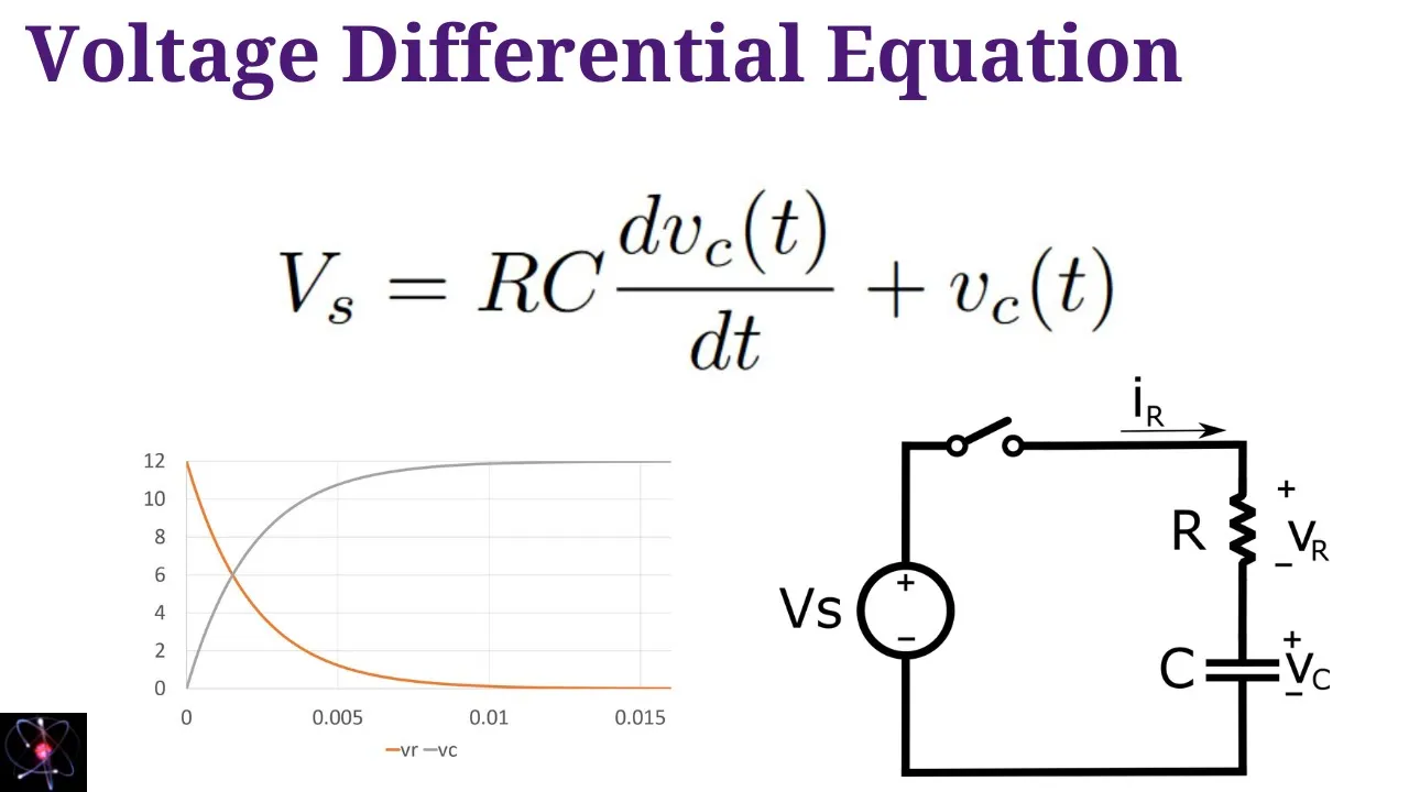
Focus on the segment from 00:00 to 02:11. This part covers the setup and derivation, which is our entire focus for today.

Let's consolidate the steps from the video into a formal derivation.

Step 1: Apply Kirchhoff's Voltage Law (KVL)

For any time $t \geq 0$ after the switch is closed, KVL tells us that the source voltage must equal the sum of the voltage drops across the resistor and the capacitor:

$V_{s} = v_{R} (t) + v_{C} (t) (1)$

This equation relates our target variable, $v_{C} (t)$ , to another time-varying function, $v_{R} (t)$ . To solve for $v_{C} (t)$ , we need to express all variables in the equation in terms of $v_{C} (t)$ and its derivatives.

Step 2: Express $v_{R} (t)$ in terms of $v_{C} (t)$

Using Ohm's law, we know that $v_{R} (t) = R \cdot i (t)$ .

Since this is a series circuit, the current $i (t)$ flowing through the resistor is the same as the current flowing through the capacitor. We can therefore use the capacitor's I-V relationship:

$i (t) = i_{C} (t) = C \frac{d v _{C} ( t )}{d t}$

Now, substitute this expression for the current back into Ohm's law for the resistor:

$v_{R} (t) = R \cdot (C \frac{d v _{C} ( t )}{d t}) = RC \frac{d v _{C} ( t )}{d t} (2)$

This is a crucial step. We have successfully expressed the voltage across the resistor in terms of the capacitor's voltage and its rate of change.

Step 3: Substitute and Form the ODE

Now we substitute our expression for $v_{R} (t)$ from equation (2) back into our KVL equation (1):

$V_{s} = RC \frac{d v _{C} ( t )}{d t} + v_{C} (t)$

This is the first-order ordinary differential equation we were looking for! It relates the function $v_{C} (t)$ to its own first derivative.

Step 4: Rearrange into Standard Form

It is conventional to write first-order linear ODEs in a standard form where the derivative term $\frac{d y}{d t}$ has a coefficient of 1. To do this, we simply divide the entire equation by the term $RC$ :

$\frac{V _{s}}{RC} = \frac{d v _{C} ( t )}{d t} + \frac{1}{RC} v_{C} (t)$

Rearranging this gives us the final standard form:

$\frac{d v _{C} ( t )}{d t} + \frac{1}{RC} v_{C} (t) = \frac{V _{s}}{RC}$

This equation is a complete mathematical model of the RC circuit's behavior over time. It states that the rate of change of the capacitor's voltage, plus a scaled version of the voltage itself, must always equal a constant determined by the source voltage and circuit components.

Conclusion

In this lesson, we successfully translated a physical circuit into a formal mathematical model. By systematically applying KVL, Ohm's law, and the capacitor's current-voltage relationship, we derived the first-order ODE that governs the charging of a capacitor in a series RC circuit.

Key Takeaways:

The behavior of an RC circuit with a step input is described by a first-order linear non-homogeneous ordinary differential equation.
The derivation relies on combining three fundamental laws: KVL, Ohm's Law, and the I-V relationship for a capacitor ( $i = C \frac{d v}{d t}$ ).
The final ODE, in standard form, is:
$\frac{d v _{C} ( t )}{d t} + \frac{1}{RC} v_{C} (t) = \frac{V _{s}}{RC}$

Preview of the Next Lesson:

We have successfully formulated the problem. The next logical step is to solve it. In the upcoming lesson, "Solving the First-Order RC Circuit ODE for its Complete Response," we will use the techniques for solving ODEs to find the function $v_{C} (t)$ that satisfies this equation and our initial condition. This will mathematically produce the exponential charging curve we discussed in our first lesson of this module.