Complete Response of RC Circuits

Hello! Welcome back to our course on radioelectronics.

In our last lesson, we successfully translated the physical RC circuit into a mathematical model, deriving its first-order ordinary differential equation (ODE). We established the "what" and the "why." Today, we'll solve that equation to find the "how"—how the capacitor's voltage actually evolves over time.

Introduction

Approximate time to complete: 45-60 minutes.

This lesson directly addresses the learning outcome: Solving the First-Order RC Circuit ODE for its Complete Response. We will take the ODE we derived previously:
$\frac{d v _{C} ( t )}{d t} + \frac{1}{RC} v_{C} (t) = \frac{V _{s}}{RC}$
and find the function $v_{C} (t)$ that satisfies it.

This process involves a standard technique for solving linear ODEs, which is a cornerstone of modeling physical systems. First, we will solve the equation from first principles to understand the underlying mathematics. Then, I'll introduce you to a powerful "engineer's shortcut" that provides an intuitive and rapid way to arrive at the same solution. This combination of rigor and practicality should resonate well with your background in both physics and software development.

1. The Complete Solution: A Tale of Two Responses

The ODE we're solving is a first-order linear non-homogeneous ODE. The term "non-homogeneous" comes from the right-hand side of the equation being non-zero ( $\frac{V _{s}}{RC}$ ). The solution to such an equation, known as the complete response, is always the sum of two components:

The Particular Integral (or Forced Response): This is the circuit's steady-state behavior. It's the voltage $v_{C} (t)$ will settle to as time approaches infinity ( $t \to \infty$ ), driven by the constant voltage source $V_{s}$ .
The Complementary Function (or Natural Response): This is the transient behavior. It describes how the circuit naturally returns to equilibrium and depends only on the circuit's components (R and C), not the external source. This part of the solution decays to zero over time.

So, our complete solution will have the form:
$v_{C} (t) = Forced Response v_{C f} (t) + Natural Response v_{C n} (t)$

The following video provides an excellent walkthrough of this entire process. We will use it to guide our derivation.

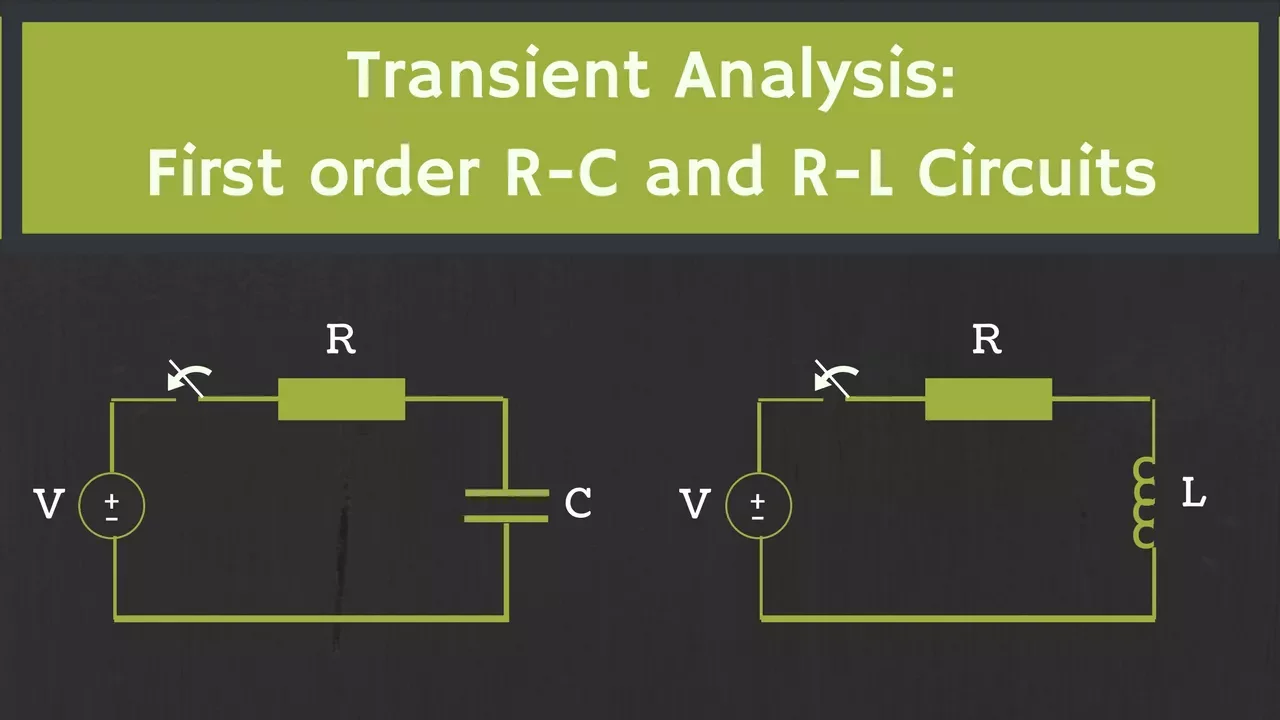
Please watch the segment from 11:16 to 15:00. This covers the setup, the separation into particular and complementary solutions, and the use of initial conditions to find the final equation. Below, I'll formalize the steps shown in the video.

Step 1: Finding the Forced Response (Particular Integral)

The forced response is the steady-state solution. After a very long time, the capacitor becomes fully charged, and current stops flowing. In this state, the capacitor acts as an open circuit.

When current stops, the voltage change across the capacitor is zero: $\frac{d v _{C}}{d t} = 0$ .
Our ODE simplifies significantly:
$0 + \frac{1}{RC} v_{C} (t) = \frac{V _{s}}{RC}$
Solving for $v_{C} (t)$ gives the steady-state voltage:
$v_{C f} (t) = V_{s}$
This is our forced response. It's a constant value that the capacitor voltage approaches.

Step 2: Finding the Natural Response (Complementary Function)

The natural response is the solution to the homogeneous version of the ODE, where we set the driving source term to zero:
$\frac{d v _{C n} ( t )}{d t} + \frac{1}{RC} v_{C n} (t) = 0$
This equation describes how the circuit would behave if left to itself. This is a separable first-order ODE, and its solution is a classic exponential decay function of the form:
$v_{C n} (t) = A \cdot e^{- t / τ}$
where $A$ is a constant we still need to find, and $τ = RC$ is the time constant of the circuit.

Step 3: Assembling the Complete Solution

Now, we sum the forced and natural responses:
$v_{C} (t) = v_{C f} (t) + v_{C n} (t) = V_{s} + A \cdot e^{- t / RC}$
This is the general form of the solution. To find the specific solution for our problem, we need to determine the constant $A$ using the circuit's initial condition.

Step 4: Applying the Initial Condition

We assume the capacitor starts with zero charge, so its initial voltage is zero: $v_{C} (0) = 0$ . Let's apply this to our general solution at $t = 0$ :
$v_{C} (0) = V_{s} + A \cdot e^{- 0/ RC}$
$0 = V_{s} + A \cdot (1)$
Solving for $A$ , we get:
$A = - V_{s}$

Step 5: The Final Equation

Substituting $A = - V_{s}$ back into our complete solution gives the final equation for the capacitor voltage:
$v_{C} (t) = V_{s} - V_{s} e^{- t / RC}$
Or, more commonly written as:
$v_{C} (t) = V_{s} (1 - e^{- t / RC})$
This is the mathematical formula describing the exponential charging curve we discussed in the first lesson of this module. It perfectly captures the behavior: at $t = 0$ , $v_{C} (0) = V_{s} (1 - 1) = 0$ , and as $t \to \infty$ , the $e^{- t / RC}$ term goes to zero, leaving $v_{C} (\infty) = V_{s}$ .

2. The Engineer's Method: A Powerful General Formula

Solving the ODE from first principles provides a solid understanding of why the solution takes its form. In practice, however, engineers often use a general formula that bypasses the formal ODE steps. This method is incredibly fast and intuitive.

The general solution for any first-order circuit (RC or RL) can be written as:

$v (t) = v (\infty) + [v (0) - v (\infty)] e^{- t / τ}$

Let's break down its components:

$v (t)$ : The value you are trying to find (voltage or current) at time $t$ .
$v (\infty)$ : The final, steady-state value after all transients have died out.
$v (0)$ : The initial value at the moment the change occurs ( $t = 0$ ).
$τ$ : The time constant of the circuit ( $τ = RC$ for an RC circuit).

Let's apply this formula to the same problem:

Final Value $v (\infty)$ : As $t \to \infty$ , the capacitor is an open circuit, so $v_{C} (\infty) = V_{s}$ .
Initial Value $v (0)$ : The capacitor starts uncharged, so $v_{C} (0) = 0$ .
Time Constant $τ$ : For our circuit, $τ = RC$ .

Plugging these into the general formula:
$v_{C} (t) = V_{s} + [0 - V_{s}] e^{- t / RC}$
$v_{C} (t) = V_{s} - V_{s} e^{- t / RC} = V_{s} (1 - e^{- t / RC})$
As you can see, we arrive at the exact same result with much less work. This method is powerful because it relies on circuit intuition (finding initial/final states) rather than formal calculus.

The following video demonstrates this exact strategy on a slightly more complex circuit, which is a great way to see it in action.

Please watch the video from 00:00 to 06:04. The instructor applies the general formula by breaking the problem down into three simple steps:

Find $V_{C} (0)$ before the switch moves.
Find $V_{C} (\infty)$ long after the switch moves.
Find the time constant $τ$ for the circuit after the switch moves.

This method is an indispensable tool for quickly analyzing first-order circuits.

Conclusion

Today we successfully solved the first-order ODE for an RC circuit, bridging the gap between a mathematical model and a predictive formula for circuit behavior.

Key Takeaways:

The complete response of a first-order circuit is the sum of its forced (steady-state) and natural (transient) responses.
By solving the ODE from first principles, we derived the capacitor charging equation: $v_{C} (t) = V_{s} (1 - e^{- t / RC})$ .
We also learned a powerful general formula for any first-order circuit: $v (t) = v (\infty) + [v (0) - v (\infty)] e^{- t / τ}$ , which relies on analyzing the circuit's initial and final states.

Preview of the Next Lesson:

Having mastered the analysis of the RC circuit, we are now ready to turn our attention to the other fundamental energy storage element: the inductor. In the next lesson, "Deriving the First-Order ODE for an RL Circuit with a Step Input," we will apply the same principles (KVL, Ohm's law, and the inductor's I-V relationship) to build a new mathematical model.