DFT Implementation and Spectral Interpretation

Hello! Welcome back to our course on Audio AI.

In our previous lesson, we completed the theoretical journey from the Continuous Fourier Transform to its practical, computable counterpart: the Discrete Fourier Transform (DFT). We derived the DFT formula, which allows us to analyze a finite sequence of digital samples and see its frequency content.

$X[k]={\sum }_{n=0}^{N-1}x[n]e^{-j\frac{2\pi kn}{N}}$

Today, we transition from theory to practice. Our goal is to implement this DFT formula from scratch and, more importantly, learn to interpret the magnitude and phase spectra it produces. This is a crucial step in moving beyond using audio analysis tools as "black boxes" and truly understanding what's happening under the hood, a key part of your goal to become an audio researcher and developer.

1. Translating the DFT Formula into an Algorithm

At its heart, the DFT formula describes a specific set of calculations. As a computer science student, you can view this as a specification for an algorithm. Let's break it down into programmable steps.

• The formula calculates an output array, $X$, of length $N$. We need to compute each element $X[k]$ for $k$ from 0 to $N-1$. This suggests an outer loop.
• Each $X[k]$ is a summation of $N$ terms, for $n$ from 0 to $N-1$. This suggests an inner loop.
• Inside the inner loop, we calculate a single term: $x[n]\cdot e^{-j\frac{2\pi kn}{N}}$. This involves complex number multiplication.

The following reading provides an excellent walkthrough of this exact translation process, from mathematical notation to imperative code.

2. A Pythonic DFT Implementation

While nested loops are a direct translation of the formula, your experience with NumPy suggests a more efficient and expressive way to implement this. The DFT can be viewed as a linear transformation, which means it can be represented by a matrix-vector multiplication.

Given the input signal vector $\vec{x}$ and the output spectrum vector $\vec{X}$, we have $\vec{X}=M\cdot \vec{x}$, where $M$ is the DFT matrix with elements:

$M_{kn}=e^{-j\frac{2\pi kn}{N}}$

This approach allows us to leverage NumPy's highly optimized routines for matrix operations, which is much faster than explicit for loops in Python. Let's look at a very clean implementation based on this idea.

This "slow" DFT implementation has a time complexity of $\mathcal{O}(N^2)$ because it involves constructing an $N\times N$ matrix and performing a matrix-vector product. We'll stick with this for now to understand the fundamentals, but keep this complexity in mind.

3. Practical Exercise: Decomposing a Signal

Now, let's put our implementation to the test. We'll create a simple signal by summing three sine waves of known frequencies and amplitudes, then use our DFT function to see if we can recover this information.

Step A: Create a Test Signal

First, we'll set up our signal parameters and generate the composite wave.

import numpy as np
import matplotlib.pyplot as plt




# Signal parameters
SAMPLING_RATE = 100  # Hertz
DURATION = 2         # Seconds
N = SAMPLING_RATE * DURATION # Number of samples




# Frequencies and amplitudes of the components
freqs = [3, 10, 18]     # Hz
amps = [2.0, 1.5, 1.0]  # Amplitudes




# Time axis
t = np.linspace(0, DURATION, N, endpoint=False)




# Create the signal by summing three sine waves
x = 0
for f, a in zip(freqs, amps):
    x += a * np.sin(2 * np.pi * f * t)




# Plot the time-domain signal
plt.figure(figsize=(12, 4))
plt.plot(t, x)
plt.title("Time-Domain Signal (Sum of 3 Sines)")
plt.xlabel("Time (s)")
plt.ylabel("Amplitude")
plt.grid(True)
plt.show()

Step B: Apply the DFT

Now, let's define our DFT_slow function and apply it to the signal x.

def dft_slow(x):
    """Compute the discrete Fourier Transform of the 1D array x"""
    x = np.asarray(x, dtype=float)
    N = x.shape[0]
    n = np.arange(N)
    k = n.reshape((N, 1))
    M = np.exp(-2j * np.pi * k * n / N)
    return np.dot(M, x)




# Compute the DFT
X = dft_slow(x)

The output X is an array of $N$ complex numbers. This is our frequency spectrum.

Step C: Interpreting the Complex Output

Each complex number $X[k]=a+bi$ in the output array holds two pieces of information about its corresponding frequency:

1. Magnitude: The magnitude, $|X[k]|=\sqrt{a^2+b^2}$, represents the strength or amplitude of that frequency component in the signal. We can calculate it with np.abs(X).
2. Phase: The phase, ${\varphi }_k=atan2(b,a)$, represents the phase shift (or starting offset) of that frequency component. We can calculate it with np.angle(X).

For many audio analysis tasks, including what we are doing now, the magnitude spectrum is of primary interest.

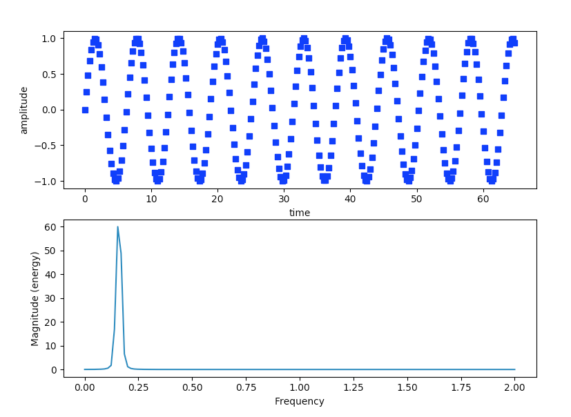
Step D: The Frequency Axis

The DFT output X is an array indexed from k = 0 to N-1. To make our plot meaningful, we must map these indices to actual frequencies in Hertz. The frequency $f_k$ corresponding to index $k$ is given by:

$f_k=k\cdot \frac{\text{Sampling Rate}}{N}$

This formula tells us that the DFT divides the entire frequency range up to the sampling rate into $N$ equally spaced "bins." The following video provides a concise explanation of this crucial relationship.

Step E: The Symmetry of the Spectrum

If you were to plot the entire magnitude spectrum, you'd notice something strange: it's perfectly symmetrical. This is a fundamental property of the DFT when applied to real-valued signals (like audio). All of the unique information is contained in the first half of the spectrum, from 0 Hz up to a special point called the Nyquist frequency, which is exactly half the sampling rate.

$f_{\text{Nyquist}}=\frac{\text{Sampling Rate}}{2}$

The second half of the spectrum is just a mirror image and can be discarded for visualization.

4. Putting It All Together: Visualization and Analysis

Let's combine everything into a final script to compute and visualize the magnitude and phase spectra of our test signal.

# We already have x and X from the previous steps




# 1. Calculate the frequency axis for the plot
# We only need the first half of the frequencies (up to Nyquist)
N_half = N // 2
freq_axis = np.linspace(0, SAMPLING_RATE / 2, N_half, endpoint=False)




# 2. Calculate magnitude and phase
# We normalize the magnitude by N/2 to get the approximate original amplitudes
magnitude = 2.0/N * np.abs(X[0:N_half])
phase = np.angle(X[0:N_half])




# 3. Plot the results
fig, (ax1, ax2) = plt.subplots(2, 1, figsize=(12, 8))




# Magnitude Plot
ax1.stem(freq_axis, magnitude)
ax1.set_title("Magnitude Spectrum")
ax1.set_xlabel("Frequency (Hz)")
ax1.set_ylabel("Amplitude")
ax1.set_xlim(0, 25) # Zoom in to see the peaks clearly
ax1.grid(True)




# Phase Plot
ax2.stem(freq_axis, phase)
ax2.set_title("Phase Spectrum")
ax2.set_xlabel("Frequency (Hz)")
ax2.set_ylabel("Phase (radians)")
ax2.set_xlim(0, 25)
ax2.grid(True)

plt.tight_layout()
plt.show()

Analysis of the Plots:
When you run this code, observe the magnitude spectrum. You should see three distinct peaks.

• Check their frequencies on the x-axis. Do they correspond to the 3 Hz, 10 Hz, and 18 Hz components we put into the signal?
• Check their amplitudes on the y-axis. Do they correspond to the 2.0, 1.5, and 1.0 amplitudes we defined? (Note: The normalization 2.0/N gives a good approximation of the original amplitudes).

The phase plot shows the initial phase of each sine wave, which should be close to -π/2 (-1.57 radians) because we used np.sin.

---

Conclusion

In this lesson, we successfully bridged the gap from the mathematical DFT formula to a working Python implementation. We've taken a signal, transformed it into the frequency domain, and interpreted the results.

Key Takeaways:

• The DFT formula can be directly translated into a nested-loop algorithm or, more efficiently in Python, a matrix-vector multiplication.
• The output of the DFT is an array of complex numbers, where the magnitude indicates the strength of a frequency component and the phase indicates its offset.
• The DFT output indices k map to physical frequencies via the formula $f_k=k\cdot (\text{Sampling Rate}/N)$.
• For real-valued input signals, the DFT spectrum is symmetric around the Nyquist frequency. We only need to analyze the first half.

The $\mathcal{O}(N^2)$ implementation we used is excellent for learning, but it's too slow for real-world audio processing where $N$ can be very large. In our next lesson, we will explore the Fast Fourier Transform (FFT), a brilliant collection of algorithms that compute the exact same DFT but with a much more efficient $\mathcal{O}(N\log N)$ complexity.