FFT vs. DFT: A Computational Efficiency Showdown

Hello! Welcome back to our journey into the world of Audio AI.

In our last lesson, we implemented a naive Discrete Fourier Transform (DFT) from scratch. We established that its computational complexity is $O (N^{2})$ , where $N$ is the number of samples. While this was great for understanding the mechanics of the DFT, this quadratic complexity poses a significant problem in practice. An audio signal just a few seconds long can have tens of thousands of samples, and an $O (N^{2})$ algorithm would be prohibitively slow.

This lesson addresses that exact problem. Our learning outcome is to explain the computational efficiency of the Fast Fourier Transform (FFT) algorithm compared to a naive DFT. You will learn that the FFT is not a different transform but a collection of highly efficient algorithms for computing the DFT. By the end, you'll understand the core "divide and conquer" strategy that reduces the complexity from $O (N^{2})$ to a much more manageable $O (N lo g N)$ .

1. The Scale of the Problem: Why $O (N^{2})$ is Unacceptable

Before diving into the solution, let's build an intuition for just how dramatic the difference between $O (N^{2})$ and $O (N lo g N)$ is.

The FFT Algorithm - Simple Step by Step

This brief clip provides a striking, tangible example of the computational savings achieved by a more efficient algorithm, illustrating why the development of the FFT was so revolutionary.

Watch the segment from 01:47 to 02:10. It presents a hypothetical scenario comparing the time required for an \mathcal{O}(N^2) operation versus an \mathcal{O}(N \log N) one. Note the staggering difference in completion time.

This massive speedup is what makes real-time audio analysis and the advanced models we'll study later in this course possible.

2. The Core Strategy: Divide and Conquer

The most famous FFT algorithm, and the one we'll focus on, is the Cooley-Tukey algorithm. Its brilliance lies in a classic computer science strategy: divide and conquer.

The key insight is that a large DFT calculation can be broken down into smaller DFT calculations. Specifically, we can split the input signal $x [n]$ into two halves: the samples at even indices and the samples at odd indices.

We can then express the original N-point DFT in terms of the DFTs of these two N/2-point signals. The following reading walks through the mathematical derivation of this process.

Radix-2 Cooley-Tukey - Divide and Conquer

Let's explore the mathematical foundation of the Cooley-Tukey algorithm. This resource from the 'Digital Signals Theory' online book provides a clear, step-by-step derivation.

Please read the introduction and the 'Divide and Conquer' section. Focus on how the single DFT summation is split into two separate summations for the even (x[2k]) and odd (x[2k+1]) parts. Pay close attention to the final equation that combines them.

As you saw in the reading, this "divide and conquer" approach results in the following fundamental relationship:

\darkblue X [m] = \magenta X_{E} [m (mod N /2)] + e^{- 2 πj \frac{m}{N}} \cdot \magenta X_{O} [m (mod N /2)]

Let's break this down:

$\darkblue X [m]$ is the desired N-point DFT output.
$\magenta X_{E}$ is the N/2-point DFT of the even-indexed samples.
$\magenta X_{O}$ is the N/2-point DFT of the odd-indexed samples.
The term $e^{- 2 πj \frac{m}{N}}$ is called a twiddle factor. It's a complex exponential that "rotates" the phase of the odd-part's DFT before it's combined with the even part.

This single equation is the heart of the FFT. It shows how to build the solution to a large DFT from the solutions of two smaller DFTs.

3. The Magic of $O (N lo g N)$ Complexity

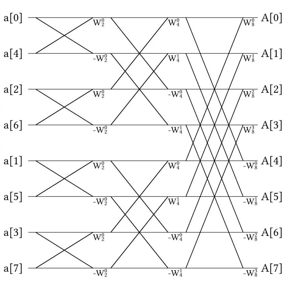
The real power emerges when we apply this "divide and conquer" strategy recursively. An N-point DFT is broken into two N/2-point DFTs. Each of those can be broken into two N/4-point DFTs, and so on, until we are left with trivial 1-point DFTs (where the DFT of a single sample is just the sample itself).

This creates a recursive structure. At each level of the recursion, we combine the results from the level below. Let's analyze the computational cost of this process.

Radix-2 Cooley-Tukey - Time analysis

Now let's formally analyze the time complexity of this recursive algorithm. This section from the same 'Digital Signals Theory' resource uses a recurrence relation to prove the \mathcal{O}(N \log N) complexity.

Read the sections 'A radix-2 algorithm' and 'Time analysis'. You don't need to memorize the Python code, but understand how it reflects the recursive structure. The key part is the 'Time analysis', which sets up and solves the recurrence relation T(N) = 2 \cdot T(N/2) + N \cdot d.

The analysis shows that we have $lo g_{2} N$ levels of recursion. At each level, we perform a total of $O (N)$ work to combine the smaller DFTs using the "twiddle factors". The total complexity is therefore the work per level times the number of levels: $O (N lo g N)$ .

The visual difference is striking.

DFT vs. FFT Run Time Comparison — This figure shows a practical comparison of run times. The naive DFT ($\mathcal{O}(N^2)$, blue line) shows a rapid, quadratic increase in computation time as the input size grows. In contrast, the FFT ($\mathcal{O}(N \log N)$, orange line) remains incredibly fast, with its run time growing almost linearly.

4. An Algorithmic Perspective: The Four Ingenious Ideas

So far, we've approached the FFT from a signal processing perspective. Given your background in computer science and algorithms, you might appreciate an alternative viewpoint that arrives at the same result. The following video frames the FFT as an ingenious solution to the problem of fast polynomial multiplication.

The Fast Fourier Transform (FFT): Most Ingenious Algorithm Ever?

This video from the YouTube channel Reducible presents one of the most elegant explanations of the FFT from a pure computer science perspective. It breaks the algorithm down into four key insights that build on each other.

Watch the video from 02:05 to 26:48. It's a bit long, but it's a masterpiece of explanation that will connect deeply with your CS background. Follow the four key ideas: Idea 1 & 2 (02:05 - 08:26): Representing polynomials by their values (points) instead of coefficients allows for fast \mathcal{O}(N) multiplication. The challenge is the conversion (evaluation), which is still \mathcal{O}(N^2). The video then introduces the recursive even/odd split. Idea 3 (08:26 - 18:33): The recursion breaks unless we can maintain a special structure in our evaluation points. This leads to the crucial insight of using complex numbers, specifically the nth roots of unity. The Algorithm (18:33 - 22:15): These ideas are synthesized into the recursive FFT algorithm. Idea 4 (22:15 - 26:48): The video reveals that the inverse operation (interpolation) uses almost the exact same algorithm, a truly beautiful result.

Both the signal processing view and the polynomial multiplication view converge on the same core mechanics: a recursive, divide-and-conquer algorithm that leverages the special properties of complex roots of unity.

The graphical representation of this computation is the famous butterfly diagram.

Radix-2 Decimation-in-Time FFT Butterfly Diagram (N=8) — An 8-point radix-2 FFT butterfly diagram. Each 'butterfly' shape represents one application of the core combination formula: $X[m] = X_E + W \cdot X_O$. The diagram visualizes the flow of data from the input samples (left, in a special 'bit-reversed' order) through the recursive stages of computation to the final DFT output (right).

5. A Crucial Point on Terminology: DFT vs. FFT

A common point of confusion is the distinction between DFT and FFT. It's vital to be precise in your language as a researcher and developer.

The Discrete Fourier Transform (DFT) is the mathematical transformation that maps a time-domain signal to its frequency-domain representation. It is the "what".
The Fast Fourier Transform (FFT) is an algorithm for computing the DFT efficiently. It is the "how".

An FFT algorithm produces a DFT. A naive $O (N^{2})$ loop also produces a DFT. The result is the same (ignoring minor floating-point precision differences); the method and its efficiency are what differ.

A Quick Rant on Word Choice

To solidify this point, please read this short, well-argued piece.

Read the section 'A Quick Rant on Word Choice'. The author's analogy to sorting algorithms (e.g., mergesort vs. the concept of 'sorting') is an excellent way for a computer scientist to frame this distinction.

Conclusion

In this lesson, we have demystified the remarkable efficiency of the Fast Fourier Transform. You now understand not just that it's faster, but why it's faster.

Key Takeaways:

A naive DFT computation has a complexity of $O (N^{2})$ , which is too slow for practical audio processing.
The FFT is an algorithm—most famously the Cooley-Tukey algorithm—that computes the DFT with a much-improved complexity of $O (N lo g N)$ .
The core strategy of the FFT is divide and conquer: recursively breaking an N-point DFT into two N/2-point DFTs and combining the results.
This recursive process relies on the special mathematical properties of the complex roots of unity to work efficiently at every level.

We now have a powerful and efficient tool for analyzing the frequency content of a signal. However, a single DFT/FFT on an entire audio clip only gives us the average frequency content over its whole duration. It doesn't tell us how those frequencies change over time. Our next lesson will introduce the Short-Time Fourier Transform (STFT), which repeatedly applies the FFT on small, overlapping windows of an audio signal to do just that.