Deriving the Discrete Fourier Transform

Hello! Welcome back to our course on Audio AI.

In our last lesson, we explored the Continuous-Time Fourier Transform (CTFT), a powerful theoretical tool that allows us to see the frequency content of a continuous signal. We established that the CTFT takes a signal from the time domain, $x(t)$, and transforms it into a continuous spectrum in the frequency domain, $X(\omega )$.

However, in the world of digital audio and computing, we don't work with continuous signals. We work with a finite number of discrete samples. The integral in the CTFT formula, which operates over infinite and continuous time, is not something we can directly compute.

This brings us to our current learning outcome: to derive the Discrete Fourier Transform (DFT) as the discrete-time counterpart of the Fourier Transform. The DFT is the practical, algorithmic workhorse of digital signal processing. It's what allows us to take a sequence of audio samples and analyze its frequency content on a computer.

This lesson will bridge the gap between the continuous theory of the CTFT and the discrete reality of the DFT.

---

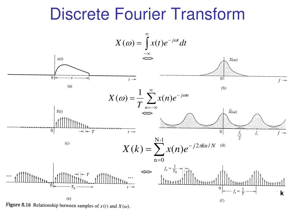
1. From Continuous Integration to Discrete Summation

The first step in moving from the continuous world to the digital one is to acknowledge that our signal isn't a continuous function $x(t)$, but a sequence of samples $x[n]$.

The CTFT is defined by an integral:

$$X(\omega )={\int }_{-\infty }^{\infty }x(t)e^{-j\omega t}dt$$

An integral is essentially a sum over an infinite number of infinitesimally small parts. When we have a finite number of discrete samples, the natural counterpart to an integral is a summation. We replace the continuous time variable $t$ with a discrete sample index $n$, and the integral $\int dt$ with a sum $\sum$.

This conceptual leap is the first step towards a computable Fourier transform. Let's watch a brief explanation that highlights this transition.

This first step of replacing the integral with a sum gives us an intermediate transform called the Discrete-Time Fourier Transform (DTFT):

$$X(\omega )=\sum _{n=-\infty }^{\infty }x[n]e^{-j\omega n}$$

Notice that while the input is discrete ($x[n]$), the output $X(\omega )$ is still a continuous function of frequency $\omega$. We can't store a continuous function in a computer. This means we're only halfway there. We need to make the frequency domain discrete as well.

The following reading provides a clear overview of the path from the theoretical continuous transforms to the practical discrete one.

---

2. Deriving the DFT: Discretizing Time and Frequency

We've established two key facts:

1. Our input signal is a sequence of $N$ discrete time samples, $x[n]$.
2. To make the output computable, we must also sample the continuous frequency spectrum at $N$ discrete frequency points.

The core idea of the DFT is to take N points in the time domain and transform them into N points in the frequency domain.

To do this, we sample the DTFT's continuous frequency axis. Since the DTFT spectrum is periodic over $2\pi$, we only need to analyze one period. We sample this $2\pi$ interval at $N$ equally spaced points. These discrete frequency "bins" are located at:

$${\omega }_k=\frac{2\pi k}{N}\text{for }k=0,1,\dots ,N-1$$

Now, we can finally derive the DFT formula by substituting these discrete frequencies ${\omega }_k$ into the DTFT equation and summing over our finite number of samples $N$. This transforms the DTFT into the DFT.

The following resource provides a rigorous, step-by-step derivation from first principles. It's a detailed and mathematically rich explanation that perfectly aligns with your goal of building a deep, foundational understanding.

By following this derivation, we arrive at the definition of the Discrete Fourier Transform (DFT):

$$X[k]=\sum _{n=0}^{N-1}x[n]e^{-j\frac{2\pi kn}{N}}\text{for }k=0,1,\dots ,N-1$$

Let's break this down:

• $x[n]$ is the $n$-th sample of our input signal.
• $N$ is the total number of samples (and also the number of frequency bins).
• $k$ is the index of the frequency bin we are calculating, from 0 up to $N-1$.
• $X[k]$ is the resulting complex number for the $k$-th frequency bin. It tells us the magnitude and phase of that frequency component.

The term $e^{-j\frac{2\pi kn}{N}}$ is particularly interesting. It is a complex exponential that represents a specific point on the unit circle in the complex plane. This is often expressed using the "twiddle factor" notation $W_N=e^{-j\frac{2\pi }{N}}$, which allows the DFT formula to be written more compactly as $X[k]={\sum }_{n=0}^{N-1}x[n]W_N^{kn}$. This forms the basis of the DFT matrix, a concept that will be very familiar from your linear algebra and computer science background.

---

3. The Inverse DFT: Reconstructing the Signal

A transform is most useful if it's reversible. The DFT is no exception. The Inverse Discrete Fourier Transform (iDFT) allows us to take the $N$ complex numbers from the frequency domain and perfectly reconstruct the original $N$ time-domain samples.

The formula is very similar, with two key differences: a scaling factor of $1/N$ and a positive sign in the exponent.

$$x[n]=\frac{1}{N}\sum _{k=0}^{N-1}X[k]e^{j\frac{2\pi kn}{N}}\text{for }n=0,1,\dots ,N-1$$

The change in sign in the exponent corresponds to "unwinding" the signal, and the $1/N$ factor normalizes the result.

The proof that the iDFT perfectly recovers the original signal relies on a property called the orthogonality of the complex exponentials. A great walkthrough of this proof is available in the Discrete–time Fourier Series and Fourier Transforms PDF by Joel Feldman, which you can find in the resources.

4. Summary: The DFT Pair

Together, the DFT and iDFT form a transform pair that allows us to move between the time and frequency domains for discrete signals.

• Forward DFT (Analysis):
  $X[k]={\sum }_{n=0}^{N-1}x[n]e^{-j\frac{2\pi kn}{N}}$
  Takes $N$ time samples $x[n]$ $\to$ Produces $N$ frequency coefficients $X[k]$.

• Inverse DFT (Synthesis):
  $x[n]=\frac{1}{N}{\sum }_{k=0}^{N-1}X[k]e^{j\frac{2\pi kn}{N}}$
  Takes $N$ frequency coefficients $X[k]$ $\to$ Reconstructs $N$ time samples $x[n]$.

This pair is the foundation of nearly all spectral analysis performed on computers.

---

Conclusion

In this lesson, we have formally derived the Discrete Fourier Transform, the essential tool for analyzing the frequency content of digital signals.

Key Takeaways:

• The DFT is the practical, computable version of the Fourier Transform, designed for finite, discrete signals (samples).
• It is derived from the theoretical CTFT by a two-step discretization process:
  1. The integral over continuous time is replaced by a sum over discrete samples.
  2. The continuous frequency axis is sampled at $N$ discrete points.
• The DFT transforms $N$ time-domain samples into $N$ complex-valued frequency-domain coefficients.
• The Inverse DFT (iDFT) perfectly reverses the process, reconstructing the original time-domain samples from the frequency coefficients.

We now have the "what" and the "why" of the DFT. In our next lesson, we will focus on the "how." We will implement a DFT from scratch in Python and learn to interpret its output, visualizing the magnitude and phase spectra that are fundamental to understanding audio signals.