Introduction to the Continuous Fourier Transform

Hello! Welcome to the first lesson of our second module, "Spectral Analysis of Audio Signals."

In the previous module, we established a solid foundation in digital audio, focusing entirely on the time domain. We learned how to represent sound as a waveform—a sequence of amplitude values over time. We manipulated these waveforms, visualized them, and even normalized them based on their temporal characteristics like peak, RMS, and perceived loudness (LUFS).

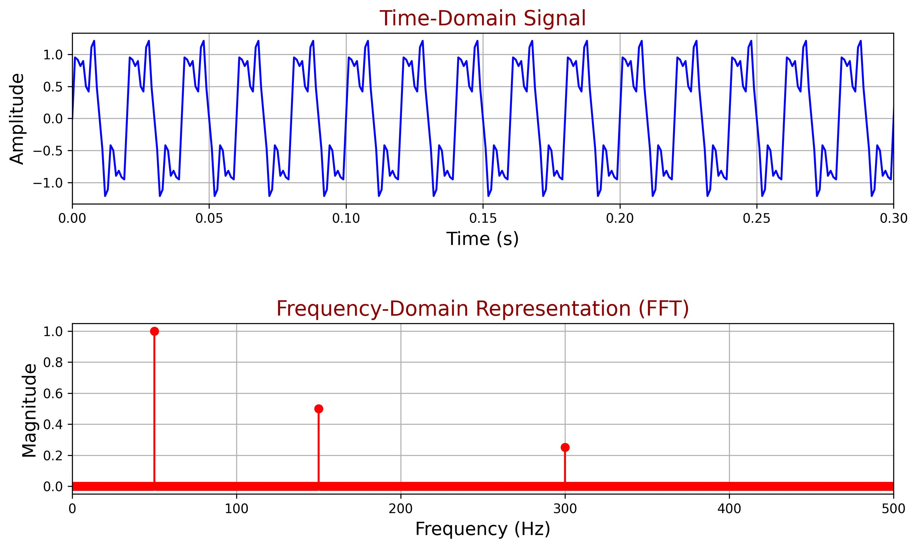
However, a time-domain view only tells us when a signal's amplitude changes. It doesn't tell us what frequencies are present in the signal. To an audio AI system, a complex vocal sound and a car engine noise are just two complicated squiggly lines. To understand what makes them different, we need to look at their frequency content.

This lesson begins our journey into the frequency domain. Our learning outcome is to define the Continuous Fourier Transform and its role in decomposing signals into frequency components. This transform is one of the most important mathematical tools in engineering and science, and it is the theoretical bedrock for almost all modern audio processing.

---

1. The Core Idea: Unmixing a Signal

At its heart, the Fourier Transform is a mathematical prism for signals. Just as a glass prism separates white light into a rainbow of individual colors (frequencies), the Fourier Transform separates a complex signal, like a sound wave, into its constituent pure frequencies.

Imagine you hear a musical chord. Your ear and brain instantly recognize it as multiple notes played together. A microphone, however, just records a single, complex pressure wave. The central question of Fourier analysis is: given that final, jumbled-up wave, how can we figure out the original notes that were played?

To build a powerful intuition for how this "unmixing" is possible, we'll start with a brilliant visual explanation.

---

2. A "Frequency-Detecting" Machine

To solve the unmixing problem, we need to build a mathematical machine that can detect the presence of a specific frequency within a complex signal. The ingenious method behind the Fourier Transform involves wrapping the signal around a circle.

Let's continue with the 3Blue1Brown video to see how this works. The key insight is that if you wrap a signal around a circle at a "winding frequency" that matches a frequency present in the signal, something special happens.

To summarize the key idea:

1. You have an input signal, $g(t)$.
2. You pick a "test frequency," $f$, that you want to search for in the signal.
3. You "wind" your signal $g(t)$ around a circle at this test frequency $f$.
4. You calculate the center of mass of this new, wound-up shape.
5. If the signal $g(t)$ contains a strong component at frequency $f$, the wound-up shape will be lopsided, and its center of mass will be far from the origin. If it contains little or no component at frequency $f$, the shape will be balanced, and its center of mass will be close to the origin.
6. By doing this for every possible test frequency $f$, you build a new plot that shows the "strength" of each frequency in the original signal. This new plot is the Fourier Transform.

---

3. From Visual Intuition to a Mathematical Formula

This "winding machine" analogy is powerful, but to use it, we need to express it mathematically. This is where complex numbers become incredibly elegant. Given your background, you'll recognize the power of using Euler's formula to describe rotation.

A point rotating clockwise around the complex plane at a frequency $f$ (in Hz) can be described by the expression $e^{-i2\pi ft}$.

Let's see how this single expression allows us to formalize the entire winding process.

This leads us to the formal definition of the Continuous-Time Fourier Transform (CTFT). Given a time-domain signal $x(t)$, its Fourier Transform $X(\omega )$ is a new function of frequency:

$$X(\omega )={\int }_{-\infty }^{\infty }x(t)e^{-j\omega t}dt$$

Let's break this down:

• $x(t)$ is our original signal as a function of time $t$.
• $\omega$ is the angular frequency in radians per second. It's the "test frequency" we're looking for. It's related to frequency $f$ in Hertz by $\omega =2\pi f$. You will see both conventions used widely.
• $e^{-j\omega t}$ is the complex exponential representing the clockwise rotation (the "winding"). The $j$ is the imaginary unit, equivalent to $i$.
• $x(t)e^{-j\omega t}$ is the value of our signal scaled by the rotation at time $t$. It represents a point on the "wound-up" graph.
• The integral ${\int }_{-\infty }^{\infty }\dots dt$ sums up all these points over all time, effectively finding the (scaled) center of mass.
• $X(\omega )$ is the result: a new function that, for any given frequency $\omega$, gives us a complex number telling us the magnitude and phase of that frequency component in the original signal.

---

4. A More Formal Derivation: From Periodic to Aperiodic

The winding analogy is a brilliant way to build intuition. The standard academic approach, common in signal processing, arrives at the same formula from a different starting point: by extending the Fourier Series.

The basic idea is:

1. The Fourier Series is a tool for decomposing periodic signals into a sum of discrete, harmonically related sine waves. The resulting spectrum is a set of spikes at integer multiples of a fundamental frequency.
2. An aperiodic signal (one that doesn't repeat) can be thought of as a periodic signal with a period $T$ that approaches infinity.
3. As the period $T\to \infty$, the fundamental frequency $f_0=1/T\to 0$. This means the discrete harmonic spikes in the spectrum get closer and closer together.
4. In the limit, as $T$ becomes infinite, the spikes merge to form a continuous spectrum. The formula describing this continuous spectrum is exactly the Fourier Transform integral.

This approach provides a rigorous mathematical bridge from representing periodic signals to representing any signal.

---

5. Understanding the Output: Magnitude and Phase

The result of the Fourier Transform, $X(\omega )$, is a complex-valued function. For any frequency $\omega$, it gives you a complex number $a+bj$. In practice, we usually don't look at the real and imaginary parts directly. Instead, we convert them to polar coordinates: magnitude and phase.

• Magnitude Spectrum $|X(\omega )|$: This tells you the "amount" or "strength" of each frequency $\omega$ in the original signal. This is what we usually visualize when we plot a "spectrum."
• Phase Spectrum $\angle X(\omega )$: This tells you the initial phase (the starting offset) of the sinusoid for each frequency $\omega$. While less intuitive, phase information is critical for perfectly reconstructing the original signal.

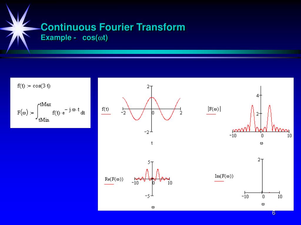
A quick note on negative frequencies: They might seem strange, but they are a natural mathematical result of using complex exponentials to represent oscillations. You can think of $e^{j\omega t}$ as a counter-clockwise rotation and $e^{-j\omega t}$ as a clockwise rotation. A real-valued sine or cosine wave is actually a combination of both, which is why its transform is symmetric around zero. For real signals, the negative frequency part is redundant, but mathematically it's always there.

---

Conclusion

In this lesson, we have defined the Continuous-Time Fourier Transform and explored its profound role in signal analysis.

Key Takeaways:

• The Fourier Transform is a mathematical tool that decomposes a signal from the time domain (amplitude vs. time) into the frequency domain (magnitude/phase vs. frequency).
• The intuitive idea behind it is to "wind" the signal around a circle at various test frequencies and measure how "lopsided" the result is to detect the strength of each frequency.
• Mathematically, this is captured by the CTFT integral: $X(\omega )={\int }_{-\infty }^{\infty }x(t)e^{-j\omega t}dt$.
• The output $X(\omega )$ is a complex function. We typically analyze its magnitude spectrum, which shows the strength of each frequency, and its phase spectrum.

The CTFT is a powerful theoretical tool that works on continuous, infinitely long signals. However, our computers work with finite, sampled audio. In our next lesson, we will bridge this gap by deriving the Discrete Fourier Transform (DFT) from the CTFT. The DFT is the practical, algorithmic version that we can actually implement in code to analyze real-world digital audio.