Classification Model Evaluation Metrics

Introduction

Hello! In our last lesson, we explored the theoretical underpinnings of model performance through the lens of the bias-variance tradeoff. You learned that a model's total error can be decomposed into bias, variance, and irreducible error, and that managing the tradeoff between bias and variance is key to building models that generalize well.

Today, we shift from theory to practice by learning how to quantify a classification model's performance. While the bias-variance framework helps us understand why a model might be failing (e.g., underfitting or overfitting), the metrics we'll cover today provide the concrete numbers to prove it.

The learning outcome for this lesson is to evaluate classification models using metrics such as accuracy, precision, recall, F1-score, and AUC-ROC. We will define each of these metrics, understand their mathematical basis, and, most importantly, explore the contexts in which each is most useful.

By the end of this lesson, you will be able to:

• Construct and interpret a confusion matrix.
• Calculate and explain accuracy, precision, recall, and the F1-score.
• Understand the precision-recall tradeoff and when to prioritize one over the other.
• Explain how the ROC curve and AUC score evaluate a model's performance across different thresholds.
• Implement these metrics using Python's scikit-learn library.

This lesson focuses on classification problems (predicting discrete categories). In the next lesson, we will cover the corresponding metrics for regression problems (predicting continuous values).

The Foundation: True Positives, False Positives, and the Confusion Matrix

Every evaluation of a binary classification model starts by comparing its predictions to the actual, ground-truth labels. This comparison results in four possible outcomes.

Let's use a common example: a model that predicts whether an email is spam (the "positive" class) or not spam (the "negative" class).

• True Positive (TP): The model correctly predicts spam, and the email is actually spam.
• True Negative (TN): The model correctly predicts not spam, and the email is actually not spam.
• False Positive (FP): The model incorrectly predicts spam, but the email is actually not spam. This is also known as a Type I Error.
• False Negative (FN): The model incorrectly predicts not spam, but the email is actually spam. This is also known as a Type II Error.

These four outcomes are typically organized into a 2x2 grid called a confusion matrix, which gives a complete picture of the model's performance.

To build a solid intuition for these concepts, please watch the first part of the following video. It provides a clear, visual explanation of these four outcomes and introduces the confusion matrix.

Now, let's explore these same concepts with a different, very concrete example. The codebasics video uses an image classification task (dog vs. not a dog) that can make these definitions feel even more tangible.

Core Performance Metrics

With the confusion matrix as our foundation, we can now define the most common evaluation metrics.

Accuracy

Accuracy is the most straightforward metric. It simply asks: "What fraction of predictions did the model get right?"

$\text{Accuracy}=\frac{\text{TP}+\text{TN}}{\text{TP}+\text{TN}+\text{FP}+\text{FN}}$

While easy to understand, accuracy can be dangerously misleading, especially when dealing with imbalanced datasets.

Imagine a credit card fraud detection model. If only 0.1% of transactions are fraudulent, a lazy model that predicts "not fraudulent" every single time will achieve 99.9% accuracy. This sounds great, but the model is completely useless because it fails to identify a single case of fraud (it has zero true positives). This is why we need more nuanced metrics.

Precision and Recall

Precision and recall are two metrics that give us a much better understanding of a model's performance, especially in the context of the positive class.

• Precision: "Of all the instances the model predicted as positive, what proportion was correct?" It measures the quality of the positive predictions.
  $\text{Precision}=\frac{\text{TP}}{\text{TP}+\text{FP}}$
  A high precision means a low false positive rate.

• Recall (or Sensitivity, or True Positive Rate): "Of all the actual positive instances, what proportion did the model correctly identify?" It measures the completeness of the positive predictions.
  $\text{Recall}=\frac{\text{TP}}{\text{TP}+\text{FN}}$
  A high recall means a low false negative rate.

Let's continue watching the video from ML & DL Explained to see how these are defined.

The Precision-Recall Tradeoff

Often, you must choose between prioritizing precision or recall. Improving one often comes at the expense of the other.

• High Precision is crucial when the cost of a False Positive is high.
  • Example: Email Spam Detection. A false positive means a legitimate email (e.g., a job offer) is sent to the spam folder. The user might miss it. We would rather let a few spam emails through (lower recall) than lose an important email.
• High Recall is crucial when the cost of a False Negative is high.
  • Example: Medical Screening for a serious disease. A false negative means a sick person is told they are healthy, and they don't get treatment. The consequences are severe. We would rather have some healthy people flagged for more tests (lower precision) than miss a sick patient.

Test your understanding!

For a model that recommends YouTube videos to users, would you prioritize precision or recall? Explain your reasoning.

Show answer

You would likely prioritize precision. A false positive here is recommending a video that the user does not like. A false negative is failing to recommend a video that the user would have liked.

The cost of a false positive (a bad recommendation) is relatively high; if the model keeps recommending irrelevant videos, the user will lose trust and stop using the service. The cost of a false negative (missing a good recommendation) is lower; there are millions of other videos, and the user won't know what they missed. Therefore, it's more important that the videos you do recommend are good (high precision).

F1-Score: A Balanced Measure

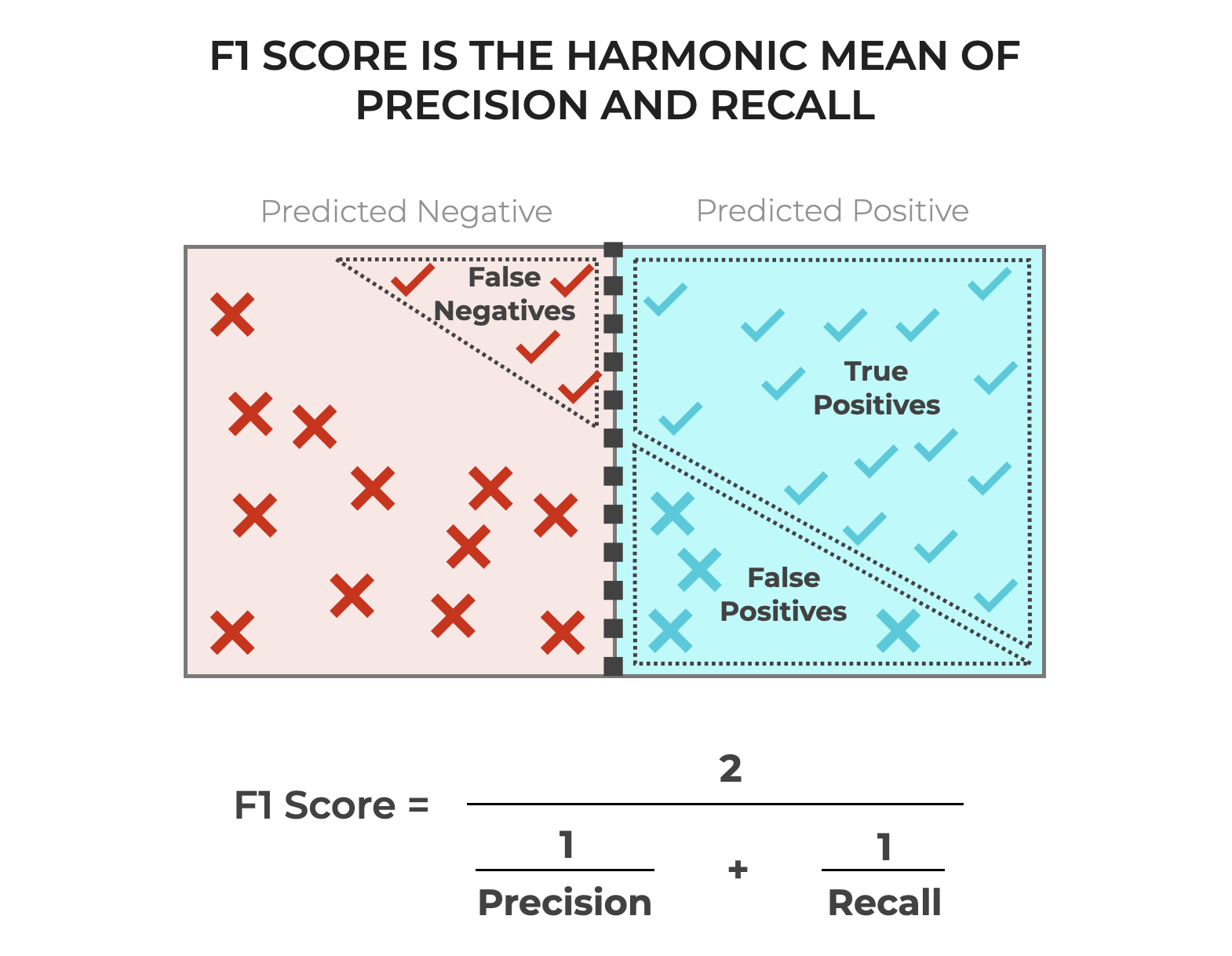
What if you need a balance between precision and recall? The F1-score is the harmonic mean of the two, providing a single score that summarizes both.

$\text{F1-Score}=2\times \frac{\text{Precision}\times \text{Recall}}{\text{Precision}+\text{Recall}}$

The F1-score is particularly useful for imbalanced datasets. Because it is a harmonic mean, it heavily penalizes models where either precision or recall is very low. A model will only get a high F1-score if both its precision and recall are high.

AUC-ROC: Evaluating Across Thresholds

Many classification models, such as logistic regression, don't just output a class label (0 or 1). Instead, they output a probability score between 0 and 1. We then use a decision threshold (typically 0.5) to convert this probability into a class prediction.

• If probability > threshold, predict 1.
• If probability <= threshold, predict 0.

Changing this threshold directly impacts our precision and recall. Lowering the threshold will increase recall (we catch more positives) but decrease precision (we make more false positive errors). The Receiver Operating Characteristic (ROC) curve is a tool that visualizes this tradeoff for every possible threshold.

The ROC curve plots two parameters:

1. True Positive Rate (TPR) on the y-axis. (This is just another name for Recall).
2. False Positive Rate (FPR) on the x-axis, calculated as:
   $\text{FPR}=\frac{\text{FP}}{\text{FP}+\text{TN}}$

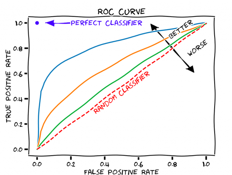
While the curve itself is informative, we often want a single number to summarize it. This is the Area Under the Curve (AUC).

• AUC = 1.0: A perfect classifier.
• AUC = 0.5: A useless classifier, equivalent to random guessing.
• AUC < 0.5: A classifier that is worse than random (you could just flip its predictions to make it better!).

The AUC has a nice probabilistic interpretation: it is the probability that the model will rank a randomly chosen positive instance higher than a randomly chosen negative instance. This makes it a great general-purpose metric for a model's ability to discriminate between classes.

Let's watch the final part of the ML & DL Explained video to see this explained.

Practical Implementation in Python

Knowing the theory is great, but in your work as a software engineer, you'll be calculating these metrics using libraries. scikit-learn makes this incredibly simple.

Let's watch the second half of the codebasics video, where he demonstrates how to generate a confusion matrix and a full classification report with just a few lines of Python.

Here's a summary of the key scikit-learn functions:

from sklearn.metrics import confusion_matrix, classification_report, roc_auc_score

# y_true: The ground-truth labels
# y_pred: The model's predicted labels
# y_pred_proba: The model's predicted probabilities for the positive class

# Example data
y_true = [0, 1, 0, 1, 1, 0, 1]
y_pred = [0, 0, 0, 1, 1, 1, 1]
y_pred_proba = [0.2, 0.4, 0.3, 0.8, 0.7, 0.6, 0.9]


# 1. Confusion Matrix
# Output is an array: [[TN, FP], [FN, TP]]
cm = confusion_matrix(y_true, y_pred)
print("Confusion Matrix:\n", cm)
# [[TN, FP],
#  [FN, TP]]
# Confusion Matrix:
#  [[2 1]
#  [1 3]]


# 2. Classification Report
# Provides precision, recall, f1-score for each class
report = classification_report(y_true, y_pred)
print("\nClassification Report:\n", report)
# Classification Report:
#                precision    recall  f1-score   support
#
#            0       0.67      0.67      0.67         3
#            1       0.75      0.75      0.75         4
#
#     accuracy                           0.71         7
#    macro avg       0.71      0.71      0.71         7
# weighted avg       0.71      0.71      0.71         7


# 3. AUC Score
# Requires the predicted probabilities, not the final class labels
auc = roc_auc_score(y_true, y_pred_proba)
print(f"\nAUC Score: {auc:.4f}")
# AUC Score: 0.8333

This classification_report is one of the most useful summary tools you'll encounter. It gives you precision, recall, and F1-score for each class, as well as overall accuracy, in a single, clean output.

Conclusion

You have now learned the essential toolkit for evaluating classification models. These metrics move us beyond simple accuracy and allow for a sophisticated, context-aware assessment of model performance.

Key Takeaways:

• The confusion matrix (TP, TN, FP, FN) is the foundation for all classification metrics.
• Accuracy is simple but can be misleading, especially on imbalanced datasets.
• Precision measures the quality of positive predictions (low FP), while Recall measures the completeness of positive predictions (low FN).
• The choice between prioritizing precision or recall depends on the real-world cost of false positives versus false negatives.
• The F1-score provides a balanced summary of precision and recall, making it a robust metric for many situations.
• The ROC curve and AUC score evaluate a model's ability to discriminate between classes across all possible decision thresholds, making it a comprehensive measure of separability.

Preview of the next lesson:
Now that you can rigorously evaluate a classifier, we'll turn our attention to its counterpart. In the next lesson, you will learn to evaluate regression models using metrics like Mean Squared Error (MSE), Mean Absolute Error (MAE), and R-squared (R²). These metrics are designed for tasks where the goal is to predict a continuous numerical value rather than a discrete category.