Understanding the Bias-Variance Tradeoff

Introduction

Hello! In our last lesson, we developed a practical toolkit for diagnosing and mitigating underfitting and overfitting. We learned to use learning curves to spot these problems and applied techniques like regularization, dropout, and early stopping to build more robust models.

Today, we will delve into the theoretical foundation that explains why these phenomena occur and why our mitigation strategies work. The learning outcome for this lesson is to analyze the bias-variance tradeoff in model complexity. We will formalize the concepts of bias and variance, which you've encountered as "underfitting" and "overfitting," and explore their inherent tension.

By the end of this lesson, you will:

Understand the formal definitions of bias, variance, and irreducible error.
Be able to explain how model complexity influences the tradeoff between bias and variance.
Appreciate the mathematical decomposition of a model's expected error into these three components.
Recognize the inherent bias-variance characteristics of different types of algorithms.

This lesson will solidify your understanding of model generalization and provide a crucial theoretical lens through which to view all future model-building and tuning efforts.

Defining Bias and Variance

In the previous lesson, we described underfitting models as having "high bias" and overfitting models as having "high variance." Let's now establish a more formal, intuitive understanding of these terms.

Bias is the error from erroneous assumptions in the learning algorithm. High bias can cause an algorithm to miss the relevant relations between features and target outputs (underfitting). It represents the systematic error of a model.
Variance is the error from sensitivity to small fluctuations in the training set. High variance can cause an algorithm to model the random noise in the training data, rather than the intended outputs (overfitting). It measures the model's instability.

A famous analogy to understand this is that of a target. Imagine the center of the target is the "true" model that we want to learn. Each time we train our model on a different subset of data, we get a slightly different set of predictions, which we can represent as a shot on the target.

Bias-Variance Tradeoff Cheat Sheet — This cheat sheet provides an excellent visual analogy. A low-bias, low-variance model consistently hits the bullseye. A high-bias model consistently misses in the same direction. A high-variance model's shots are scattered all over the place.

To solidify these definitions, let's explore them through a clear, concise article.

Mastering the Bias-Variance Tradeoff in Machine Learning

The article 'Mastering the Bias-Variance Tradeoff' on the Lightly AI blog offers excellent, clear-cut definitions of these concepts.

Please read the 'Quick answers' (TL;DR) section at the top, followed by the sections 'What is Bias in Machine Learning?', 'What is Variance in Machine Learning?', and 'Underfitting vs Overfitting'. This will provide a solid conceptual foundation.

The Tradeoff and Model Complexity

The central challenge in model selection is that bias and variance are often at odds with each other.

A simple model (e.g., linear regression, low-degree polynomial) has high bias because its assumptions are too rigid. However, it has low variance because it doesn't change much if you train it on different subsets of data.
A complex model (e.g., a deep neural network, high-degree polynomial) has low bias because it's flexible enough to capture intricate patterns. However, it has high variance because it's so flexible that it can model the specific noise of any given training set.

This inverse relationship is the bias-variance tradeoff. Our goal is not to eliminate one or the other, but to find a sweet spot in model complexity that minimizes the total error.

Let's see this in action. The following video provides an intuitive demonstration using polynomial regression, which you might recall from our discussion on overfitting.

Machine Learning-Bias And Variance In Depth Intuition| Overfitting Underfitting

This video by Krish Naik clearly demonstrates how changing model complexity (the degree of the polynomial) directly impacts bias and variance, leading to underfitting and overfitting.

Watch from 00:36 to 07:21, and then from 09:24 to 12:33. The first part shows the polynomial regression example. The second part presents the general graphical representation of the tradeoff, which is a key visual to understand.

As the video illustrates, as model complexity increases, the training error consistently goes down. The test error, however, follows a characteristic U-shape. This curve represents the sum of the decreasing bias and the increasing variance.

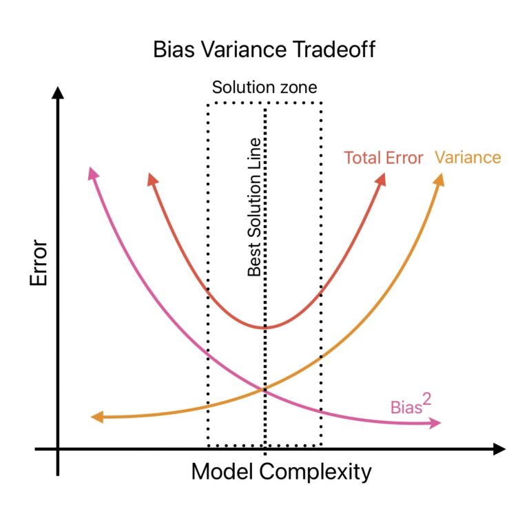
Bias-Variance Tradeoff Graph — This graph visualizes the core of the tradeoff. As model complexity increases, bias squared (Bias²) decreases while variance increases. The total error, their sum, reaches a minimum at an optimal level of complexity.

Test your understanding!

In the previous lesson, we discussed L2 regularization, where we add a penalty term $λ \sum w_{i}^{2}$ to the loss function. A larger $λ$ penalizes model complexity more heavily.

On the graph above, would increasing the value of $λ$ move our model to the left or to the right on the "Model Complexity" axis? What would be the expected effect on bias and variance?

Show answer

Increasing $λ$ would move our model to the left on the Model Complexity axis. This is because a larger penalty forces the model to be simpler (smaller weights). The expected effect would be an increase in bias (as the model becomes less flexible) and a decrease in variance (as the model becomes less sensitive to the training data). This is precisely how regularization helps combat overfitting (high variance).

The Mathematical Decomposition of Error

This U-shaped curve isn't just an empirical observation; it can be mathematically derived. The total expected error of a supervised learning model, typically measured by Mean Squared Error (MSE), can be decomposed into three distinct components.

Total Error = Bias² + Variance + Irreducible Error

Let's break down the new term:

Irreducible Error ( $σ^{2}$ ): This is the error caused by inherent noise or randomness in the data itself. It's the lower bound on the error that any model can achieve. We can't reduce this error by choosing a better model; it's a property of the data.

Now, let's go through the formal decomposition. Given your computer science and mathematics background, you should find the derivation insightful. It shows precisely how these components emerge from the definition of expected squared error.

What is Bias-Variance Tradeoff?

The article 'What is Bias-Variance Tradeoff?' by IBM provides a very clean and step-by-step derivation of the bias-variance decomposition.

Please read the section 'Theoretical foundations'. Follow the derivation from the initial expression for expected prediction error, through the expansion and final decomposition. Don't worry about memorizing every step, but focus on understanding how the final three terms are separated out.

Let's formalize the final result. For a given test point $x$ , if the true function is $y = f (x) + ϵ$ (where $ϵ$ is noise with mean 0 and variance $σ^{2}$ ) and our model is $\hat{f} (x)$ , the expected squared prediction error is:

E [(y - \hat{f} (x))^{2}] = Bias^{2} (E [\hat{f} (x)] - f (x))^{2} + Variance E [(\hat{f} (x) - E [\hat{f} (x)])^{2}] + Irreducible Error σ^{2}

The Bias² term measures how far the average prediction of our model (over all possible training sets) is from the true value.
The Variance term measures the expected squared deviation of any single model's prediction from that average prediction. It captures the model's instability.
The Irreducible Error is the variance of the noise term $ϵ$ , which is beyond our control.

The Tradeoff in Practice: Algorithms and Techniques

Understanding this decomposition allows us to classify algorithms and techniques by how they manage the tradeoff.

What is Bias-Variance Tradeoff?

Let's return to the IBM article to see how this theory connects to the practical methods we discussed in the last lesson.

Read the sections 'Real-world consideration' and 'Applications to modern AI'. This will explicitly connect techniques like regularization and ensemble methods (bagging, boosting) to their effects on bias and variance. The discussion on CNNs and RNNs also provides a great preview for future modules.

Different algorithms also have their own inherent bias-variance characteristics. Knowing these tendencies can help you choose a good starting point for a given problem.

Algorithm	Inherent Tendency	Characteristics
Linear Regression	High Bias, Low Variance	Assumes a linear relationship. Stable but can't capture complex patterns.
Decision Tree (unpruned)	Low Bias, High Variance	Very flexible and can fit any data, but is highly unstable and prone to overfitting.
k-Nearest Neighbors (k-NN)	Tunable	Small `k` leads to high variance, low bias. Large `k` leads to low variance, high bias.
Bagging (e.g., Random Forest)	Low Bias, Lowered Variance	Averages many high-variance models (trees) to reduce variance while keeping bias low.
Boosting (e.g., GBM, XGBoost)	Reduced Bias, Controlled Variance	Sequentially builds models to correct the errors of previous ones, primarily reducing bias.
Neural Networks (large)	Low Bias, High Variance (potential)	Extremely flexible (low bias). High variance is managed with large datasets and regularization (dropout, L2).

(This table is adapted from the Lightly AI article "Mastering the Bias-Variance Tradeoff")

This table crystallizes why, for example, a Random Forest (an ensemble of decision trees) is often a much better out-of-the-box performer than a single, large decision tree. It's a direct practical consequence of managing the bias-variance tradeoff.

Conclusion

Today, you have connected the practical issues of overfitting and underfitting to their theoretical source: the bias-variance tradeoff. This framework is fundamental to the art and science of machine learning.

Key Takeaways:

A model's total error can be decomposed into Bias², Variance, and Irreducible Error.
Bias is a systematic error from a model being too simple (underfitting).
Variance is an error from model instability and sensitivity to the training data (overfitting).
There is an inherent tradeoff: decreasing bias by increasing model complexity typically increases variance, and vice-versa.
The goal of model tuning is to find the "sweet spot" of complexity that minimizes the total error, not just one of its components.
Techniques like regularization and ensembling are practical tools for managing this tradeoff.

Preview of the next lesson:
We have now completed our foundational module on Core Machine Learning Concepts. You have a solid grasp of model evaluation, diagnostics, and complexity control. We are perfectly positioned to begin Module 3: Classical and Ensemble Learning Algorithms. In our next lesson, we will implement linear regression, the quintessential high-bias, low-variance model. We will then immediately apply L1 and L2 regularization to it, allowing you to see firsthand how these techniques control variance in one of machine learning's foundational algorithms.