Self-Attention: Beyond Recurrence for Long-Range Dependencies

Hello! Welcome to the third lesson in our module on Sequence Modeling.

In our last lesson, we explored RNNs and LSTMs, architectures designed to process sequences by maintaining a "memory" through a hidden state. We saw how LSTMs, with their gating mechanisms and cell state, provided a powerful solution to the vanishing gradient problem that plagued simple RNNs. However, we also noted a fundamental bottleneck: their sequential nature. To process the 100th element in a sequence, an LSTM must first process the preceding 99, making parallelization impossible and still posing challenges for capturing extremely long-range dependencies.

Today, we will explore a mechanism that revolutionized sequence modeling by breaking free from this sequential constraint. The learning outcome for this lesson is to: Explain the self-attention mechanism and its advantages over recurrent models for capturing long-range dependencies. We will dissect the celebrated "Attention Is All You Need" paradigm, understanding its components and why it has become the foundation of modern models like the Transformer.

1. The Inherent Limitations of Recurrence

Before we dive into the solution, let's crystallize the problems with recurrent architectures that motivated the search for an alternative. Even powerful variants like LSTMs face challenges when dealing with very long sequences.

To understand these limitations better, let's watch a brief segment from an MIT lecture that summarizes the core issues.

As the video highlights, the core problems are:

1. Information Bottleneck: The fixed-size hidden state vector $h_t$ must compress the entire history of the sequence up to time $t$. For long sequences, this is an aggressive form of compression that can lead to information loss.
2. Sequential Computation: The calculation of $h_t$ depends on $h_{t-1}$, meaning the computations cannot be parallelized across the time dimension. This makes RNNs slow to train on long sequences.
3. Path Length: To connect two distant elements in a sequence, information (and gradients during training) must travel through all intermediate steps. The path length between elements at positions $i$ and $j$ is proportional to $|i-j|$. This long path makes it difficult for the model to learn relationships between distant parts of a sequence.

Self-attention was developed to solve these three problems simultaneously.

2. The Core Idea: Attention as Weighted Information Retrieval

At its heart, attention is an intuitive concept. When you listen to someone speak, you don't give equal weight to every word; you focus on the words that are most relevant to understanding the current thought. The attention mechanism brings this idea into neural networks.

Instead of forcing a model to cram all information into a single state, attention allows the model to look at the entire input sequence at once and, for each element it's processing, decide which other elements are most important.

Let's watch a video from 3Blue1Brown that provides a superb high-level intuition for why this is so powerful.

The key takeaway is that attention provides a mechanism to create context-aware representations. The initial embedding for "mole" is generic; attention allows the model to pull in information from "shrew" or "carbon dioxide" to produce a new, contextually refined embedding.

3. The Self-Attention Mechanism: Queries, Keys, and Values

How does a model "decide" what's important? Self-attention formalizes this using an analogy from information retrieval systems: a query, keys, and values.

Imagine you're searching a database (like YouTube):

• You have a Query (your search term, e.g., "deep learning introduction").
• The database has Keys for each item (video titles). You compare your query to each key to find a match.
• Each item also has a Value (the video content itself). Once you find the best match based on the key, you retrieve the corresponding value.

Self-attention applies this concept to a sequence of input vectors (e.g., word or audio embeddings). For each element in the sequence, it generates three vectors:

1. Query ($\mathbf{q}$): "I am element $i$. What kind of information am I looking for to better understand myself?"
2. Key ($\mathbf{k}$): "I am element $j$. This is the kind of information I offer."
3. Value ($\mathbf{v}$): "I am element $j$. This is the actual information I contain."

The process works as follows: to update itself, each element's Query is compared against every other element's Key. The compatibility scores are used to create a weighted sum of all the Values in the sequence.

Let's formalize this with the mathematics.

Step 1: Create Query, Key, and Value Vectors

We start with an input sequence of embeddings, let's call it $\mathbf{X}\in {\mathbb{R}}^{n\times d_{\text{model}}}$, where $n$ is the sequence length and $d_{\text{model}}$ is the embedding dimension.

To get the Q, K, and V vectors, we create three learnable weight matrices: ${\mathbf{W}}^Q$, ${\mathbf{W}}^K$, and ${\mathbf{W}}^V$. We then multiply our input matrix $\mathbf{X}$ by these matrices:

$$\mathbf{Q}=\mathbf{X}{\mathbf{W}}^Q$$ $$\mathbf{K}=\mathbf{X}{\mathbf{W}}^K$$ $$\mathbf{V}=\mathbf{X}{\mathbf{W}}^V$$

The weight matrices ${\mathbf{W}}^Q,{\mathbf{W}}^K\in {\mathbb{R}}^{d_{\text{model}}\times d_k}$ and ${\mathbf{W}}^V\in {\mathbb{R}}^{d_{\text{model}}\times d_v}$ are learned during training. They project the input embeddings into three distinct spaces for querying, matching, and information retrieval.

Step 2: Calculate Attention Scores

To find out how much each element should "attend" to every other element, we compute a score. For a query vector ${\mathbf{q}}_i$ from position $i$ and a key vector ${\mathbf{k}}_j$ from position $j$, the score is their dot product. This is calculated for all pairs, forming a score matrix $\mathbf{S}$.

$$\mathbf{S}=\mathbf{Q}{\mathbf{K}}^T$$

An element $S_{ij}$ in this matrix represents the similarity or relevance of element $j$ to element $i$.

Step 3: Scale the Scores

A crucial, yet subtle, step is to scale the scores. The authors of "Attention Is All You Need" found that for large values of $d_k$, the dot products could grow very large in magnitude. This pushes the softmax function (our next step) into regions with extremely small gradients, making learning difficult.

To counteract this, they scale the scores by dividing by the square root of the dimension of the key vectors, $d_k$.

$$\text{Scaled Scores}=\frac{\mathbf{Q}{\mathbf{K}}^T}{\sqrt{d_k}}$$

For a deeper look into the mathematical justification for this scaling factor, I recommend reading the following resource. It formally proves that this scaling ensures the scores maintain a variance of 1, which helps stabilize training.

Step 4: Normalize with Softmax

Next, we apply a softmax function along each row of the scaled score matrix. This converts the scores into a probability distribution, giving us the attention weights, denoted by $\mathbf{A}$.

$$\mathbf{A}=\text{softmax}\left(\frac{\mathbf{Q}{\mathbf{K}}^T}{\sqrt{d_k}}\right)$$

Each element $A_{ij}$ is now a value between 0 and 1, and the sum of each row is 1. $A_{ij}$ represents the weight or importance of value vector ${\mathbf{v}}_j$ when constructing the new representation for element $i$.

Step 5: Produce the Output

Finally, we compute the output of the self-attention layer by taking a weighted sum of the value vectors, using the attention weights we just calculated.

$$\text{Output}(\mathbf{Q},\mathbf{K},\mathbf{V})=\mathbf{AV}$$

The output for position $i$, ${\mathbf{y}}_i$, is ${\sum }_{j=1}^n{A}_{ij}{\mathbf{v}}_j$. It's a new representation of element $i$ that has been enriched with contextual information from the entire sequence, weighted by relevance.

The following video provides an excellent visual walkthrough of this entire process, from creating Q, K, V to the final weighted sum.

4. Advantages of Self-Attention Over Recurrent Models

Now that we understand the mechanism, let's explicitly state its advantages over RNNs/LSTMs.

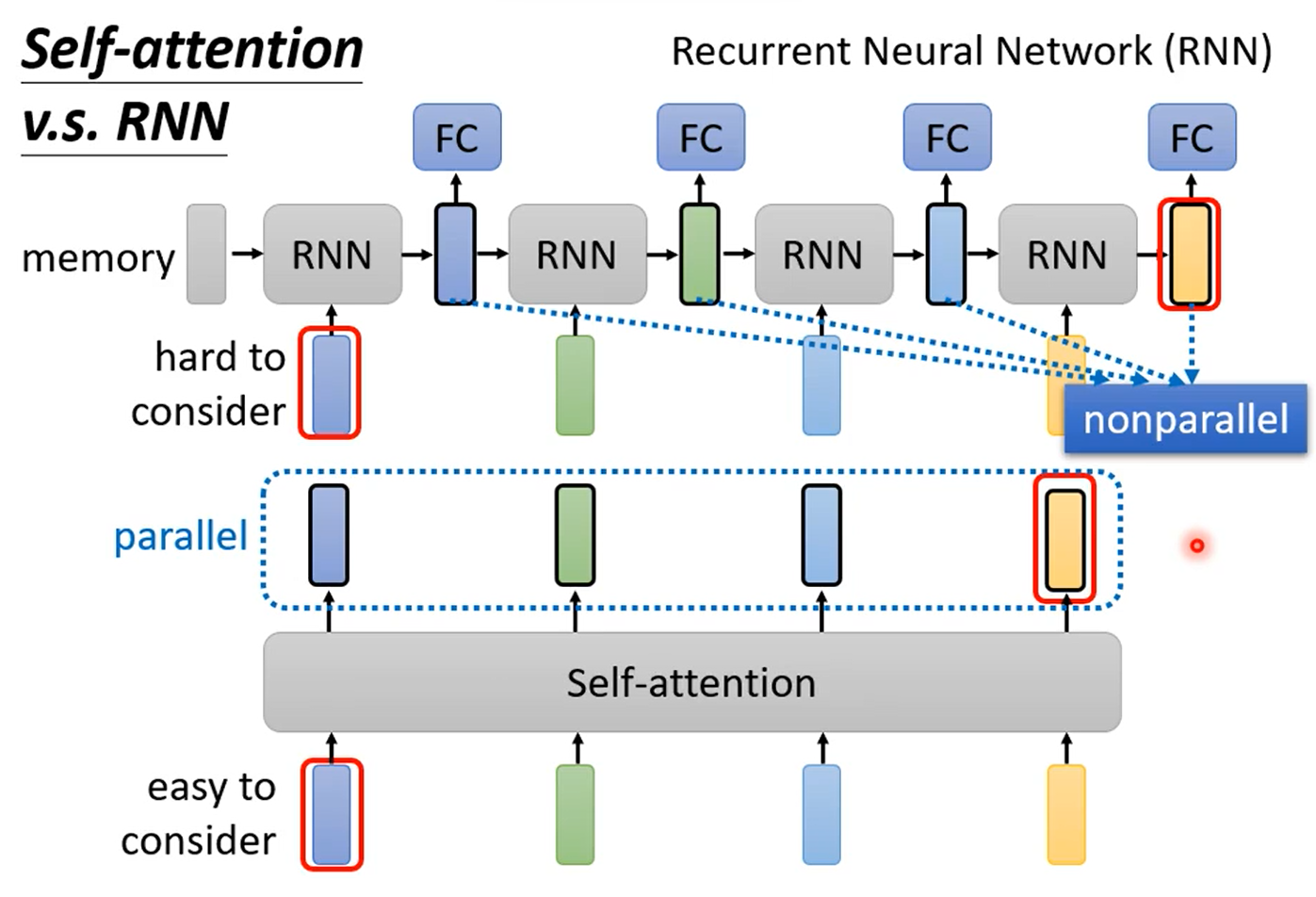
1. Direct Connections and Shorter Path Length: This is the most significant advantage for capturing long-range dependencies. In self-attention, the path length between any two tokens in the sequence is $O(1)$. They are connected directly through the attention matrix. In an RNN, the path length is $O(n)$, where $n$ is the distance between the tokens. The shorter path in self-attention allows gradients to flow directly between distant tokens, making it much easier to learn long-range relationships and mitigating the vanishing gradient problem far more effectively than even LSTMs.

2. Parallelizability: The computation for each position in the sequence is independent of the others (within a single layer). The matrix multiplications $\mathbf{Q}{\mathbf{K}}^T$ and $\mathbf{AV}$ can be computed for all positions simultaneously. This allows for massive parallelization on modern hardware like GPUs and TPUs, leading to significantly faster training times compared to the inherently sequential nature of RNNs.

3. Computational Complexity Trade-off: The computational complexity per layer is also different.

   • Self-Attention: $O(n^2\cdot d)$, where $n$ is sequence length and $d$ is dimension. The complexity is quadratic in sequence length but linear in dimension.
   • RNN/LSTM: $O(n\cdot d^2)$. The complexity is linear in sequence length but quadratic in dimension.

For shorter sequences where $n<d$ (which is common, e.g., a 512-token sequence with a 768-dim embedding), self-attention is computationally more efficient per layer. However, the $n^2$ complexity becomes a bottleneck for very long sequences, a problem that has spurred much research into more efficient attention variants.

The following resource provides a table that neatly summarizes this comparison.

5. A Final Note on Positional Information

There's one "catch" with self-attention as we've described it: the mechanism is permutation invariant. If you shuffle the input sequence, the attention scores between any two words will be the same, and the final output (when shuffled back) will also be the same. The model has no inherent sense of word order.

To fix this, Transformers inject information about the position of each token into the input embeddings. This is done using positional encodings. These are vectors that are added to the input embeddings to give the model a sense of sequence order. We will delve into these in the next lesson when we assemble the full Transformer architecture.

Conclusion

In this lesson, we dismantled the self-attention mechanism and contrasted it with the recurrent models we studied previously. It represents a fundamental shift from sequential processing to parallel, fully-connected information retrieval.

Key Takeaways:

• Self-attention computes a new representation for each token in a sequence by taking a weighted sum of all other tokens' representations.
• The mechanism is based on Queries, Keys, and Values (Q, K, V), which are learned projections of the input embeddings.
• Attention weights are calculated by taking the softmax of the scaled dot-product of queries and keys.
• The primary advantages over RNNs/LSTMs are:
  • $O(1)$ maximum path length, enabling superior learning of long-range dependencies.
  • High parallelizability, leading to faster training and inference.
• The main drawback is its $O(n^2)$ computational complexity with respect to sequence length $n$.
• Self-attention is order-agnostic and requires positional encodings to be aware of sequence order.

Preview of the Next Lesson:
Self-attention is just one (albeit crucial) component. A full Transformer model combines it with other key pieces. In the next lesson, we will explore Multi-Head Attention, where multiple attention mechanisms run in parallel to capture different types of relationships, and see how it fits together with positional encoding and feed-forward layers to form the complete Transformer architecture.