RNN and LSTM Architectures for Temporal Sequences

Hello! Welcome to the second lesson in our module on Sequence Modeling.

In the previous lesson, we established how 1D Convolutional Neural Networks (CNNs) serve as powerful feature extractors for raw audio. We saw that their strength lies in detecting local patterns through learned filters. However, a CNN's view is inherently local, limited by its receptive field. Tasks like speech recognition require understanding context over much longer time scales—how a word spoken now relates to one spoken several seconds earlier.

This brings us to today's topic. We will address the learning outcome: Describe the architecture of Recurrent Neural Networks (RNNs) and LSTMs for modeling temporal sequences. We will explore the classic architectural solution for modeling sequences, understanding its core mechanism, its fundamental limitations, and the powerful variant that dominated sequence modeling for years: the LSTM.

1. The Idea of Recurrence

To process a sequence, a model needs a sense of memory. It needs to know not just the current input, but also what came before it. The core idea of a Recurrent Neural Network is to achieve this through a loop. An RNN processes a sequence one element at a time, and at each step, it uses not only the current input but also an internal hidden state, which is a summary of all the previous steps.

Let's watch a segment of a lecture from Stanford University that introduces this concept and its applications.

The key idea is that the network applies the same set of operations at every time step, constantly updating its hidden state. This makes it a very efficient way to process sequences of any length.

2. The "Vanilla" RNN Architecture

The most intuitive way to understand the data flow in an RNN is to "unroll" it through time. Instead of a diagram with a loop, we can visualize it as a chain of identical network modules, where each module passes its hidden state to the next one in the sequence.

Let's look at the mathematics of this unrolled chain.

As the video explains, the core of the RNN is defined by two equations:

1. Hidden State Update: The hidden state $h_t$ at time step $t$ is a function of the input at that time step, $x_t$, and the hidden state from the previous time step, $h_{t-1}$.

   $$h_t=\tanh (W_{hh}{h}_{t-1}+W_{xh}{x}_t+b_h)$$

2. Output: The output $y_t$ at time step $t$ is typically a function of the hidden state at that same time step.

   $$y_t=W_{hy}{h}_t+b_y$$

Here's a breakdown of the components:

• $x_t$: The input vector at time step $t$ (e.g., a feature vector from our CNN encoder).
• $h_t$: The hidden state vector at time step $t$. It's the network's "memory."
• $y_t$: The output vector at time step $t$.
• $W_{xh}$, $W_{hh}$, $W_{hy}$: Weight matrices that are shared across all time steps. These are the parameters the network learns.
• $b_h$, $b_y$: Bias vectors, also shared across time.
• tanh: The hyperbolic tangent activation function, which squashes the values into the range [-1, 1].

The concept of parameter sharing is fundamental. The network doesn't learn a separate set of weights for each time step. It learns a single set of weights ($W_{xh}$, $W_{hh}$, $W_{hy}$) that is applied repeatedly. This is what allows an RNN to generalize to sequences of varying lengths and makes it incredibly parameter-efficient.

3. The Problem: Unstable Gradients

Training an RNN involves a process called Backpropagation Through Time (BPTT). Because the output at a given time step depends on computations from all previous time steps, the gradients must be propagated "back through time" all the way to the beginning of the sequence.

Let's see why this poses a significant problem.

The issue stems from the chain rule being applied repeatedly through the recurrent connections. To calculate the gradient of the loss with respect to an early hidden state $h_k$, we have to backpropagate through all the intermediate steps from $h_t$ down to $h_k$.

At each step backward, the gradient is multiplied by the transpose of the recurrent weight matrix, $W_{hh}^T$. So, for a long sequence, the gradient calculation involves multiplying by this matrix many times:

This leads to two scenarios:

1. Exploding Gradients: If the singular values of the $W_{hh}$ matrix are greater than 1, repeated multiplication causes the gradient values to grow exponentially, leading to huge, unstable weight updates. This is often addressed with a simple but effective hack called gradient clipping, where gradients are capped at a certain threshold.
2. Vanishing Gradients: If the singular values of $W_{hh}$ are less than 1, repeated multiplication causes the gradients to shrink exponentially toward zero. This is a more insidious problem. It means the network is unable to learn long-range dependencies because the influence of early time steps effectively vanishes by the time the gradient signal reaches them.

The vanishing gradient problem severely limits the "memory" of a vanilla RNN, making it difficult to capture relationships spanning more than a few time steps. This was a major roadblock for sequence modeling until a more sophisticated architecture was developed.

4. The Solution: Long Short-Term Memory (LSTM)

The Long Short-Term Memory (LSTM) network, proposed by Hochreiter & Schmidhuber in 1997, was designed specifically to combat the vanishing gradient problem. It introduces a more complex internal structure that allows information to flow more effectively over long durations.

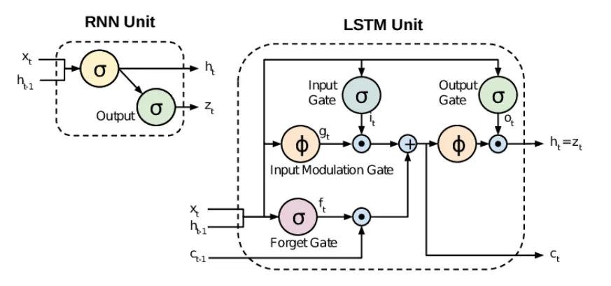
The key innovation of the LSTM is the cell state, which you can think of as a "conveyor belt" of information. The LSTM can read from, write to, and reset this cell state via three mechanisms called gates.

To understand the gates and the mathematical operations, let's consult a detailed article.

Let's summarize the components of an LSTM cell at a time step $t$:

• Inputs: Current input $x_t$, previous hidden state $h_{t-1}$, previous cell state $C_{t-1}$.
• Outputs: Current hidden state $h_t$, current cell state $C_t$.

The operations are as follows:

1. Forget Gate ($f_t$): Decides what information to throw away from the previous cell state $C_{t-1}$. It looks at $h_{t-1}$ and $x_t$ and outputs a number between 0 and 1 for each component of the cell state vector. A 1 means "keep it," and a 0 means "forget it."

   $$f_t=\sigma (W_f[h_{t-1},x_t]+b_f)$$

2. Input Gate ($i_t$) & Candidate State (${\tilde{C}}_t$): Decides what new information to store in the cell state.

   • The input gate ($i_t$) uses a sigmoid to decide which values to update.
   • The candidate state (${\tilde{C}}_t$) uses a tanh to create a vector of new candidate values that could be added.
   $$i_t=\sigma (W_i[h_{t-1},x_t]+b_i)$$ $${\tilde{C}}_t=\tanh (W_C[h_{t-1},x_t]+b_C)$$

3. Cell State Update: The old cell state $C_{t-1}$ is updated to the new cell state $C_t$. The old state is multiplied by the forget gate, and then we add the product of the input gate and the candidate state.

   $$C_t=f_t\odot C_{t-1}+i_t\odot {\tilde{C}}_t$$

   (Note: $\odot$ denotes element-wise multiplication.)

4. Output Gate ($o_t$): Decides what to output as the hidden state $h_t$.

   • First, a sigmoid layer decides which parts of the cell state we're going to output.
   • Then, the cell state is passed through tanh to push the values to be between -1 and 1 and multiplied by the output of the sigmoid gate.
   $$o_t=\sigma (W_o[h_{t-1},x_t]+b_o)$$ $$h_t=o_t\odot \tanh (C_t)$$

How LSTMs Mitigate Vanishing Gradients

The magic lies in the cell state update equation: $C_t=f_t\odot C_{t-1}+i_t\odot {\tilde{C}}_t$.

Notice that this operation is primarily additive. During backpropagation, the gradient with respect to the cell state flows back through this addition. Unlike the vanilla RNN which involved repeated matrix multiplication, the gradient flow through the LSTM's cell state is much more direct. It's an uninterrupted "gradient superhighway" where gradients can pass through long sequences without vanishing. The forget gate's element-wise multiplication can still scale the gradient, but the model can learn to set the forget gate's values close to 1.0 to preserve the gradient signal.

Conclusion

In this lesson, we have explored the foundational recurrent architectures for sequence modeling. We started with the simple, elegant concept of an RNN and discovered its critical flaw, before moving on to the more robust LSTM.

Key Takeaways:

• RNNs process sequences by maintaining a hidden state that is updated at each time step, allowing them to have "memory." Their use of parameter sharing makes them efficient for variable-length inputs.
• Vanishing/Exploding Gradients are a major problem in vanilla RNNs due to the repeated multiplication of gradients with the recurrent weight matrix during Backpropagation Through Time. This limits their ability to learn long-range dependencies.
• LSTMs solve this problem with a more sophisticated architecture featuring a dedicated cell state and three gates (forget, input, output).
• The gates regulate the flow of information, allowing the LSTM to selectively remember or forget information over long durations.
• The additive nature of the cell state update creates a "gradient superhighway," enabling gradients to flow across many time steps without vanishing, which is the key to learning long-term dependencies.

Preview of the Next Lesson:
LSTMs were the state-of-the-art for many years, but they still have a fundamental bottleneck: they must process sequences sequentially, one step at a time. In the next lesson, we will introduce the self-attention mechanism, a powerful idea that allows a model to look at all parts of a sequence simultaneously and weigh their importance. This concept is the heart of the Transformer architecture and the key to its revolutionary success.