Deconstructing the Transformer Architecture

Hello! Welcome to the fourth lesson in our module on Sequence Modeling.

In our last lesson, we took a deep dive into the self-attention mechanism, the engine that powers the Transformer. We saw how it uses Queries, Keys, and Values to create context-aware representations, and we highlighted its key advantages over RNNs: direct, $O(1)$ path lengths between any two tokens and massive parallelizability.

However, we also left a loose end: self-attention, by itself, is permutation invariant—it has no inherent sense of word order. We also only looked at it in isolation. Today, we'll address that and assemble the complete puzzle.

The learning outcome for this lesson is to: Describe the complete Transformer architecture, including positional encoding, multi-head attention, and feed-forward layers. We will construct the model brick by brick, from the input embeddings to the final output probabilities, understanding how each component contributes to the whole.

1. The Transformer: A High-Level View

At its core, the Transformer maintains the familiar encoder-decoder structure common in sequence-to-sequence tasks like machine translation or speech recognition.

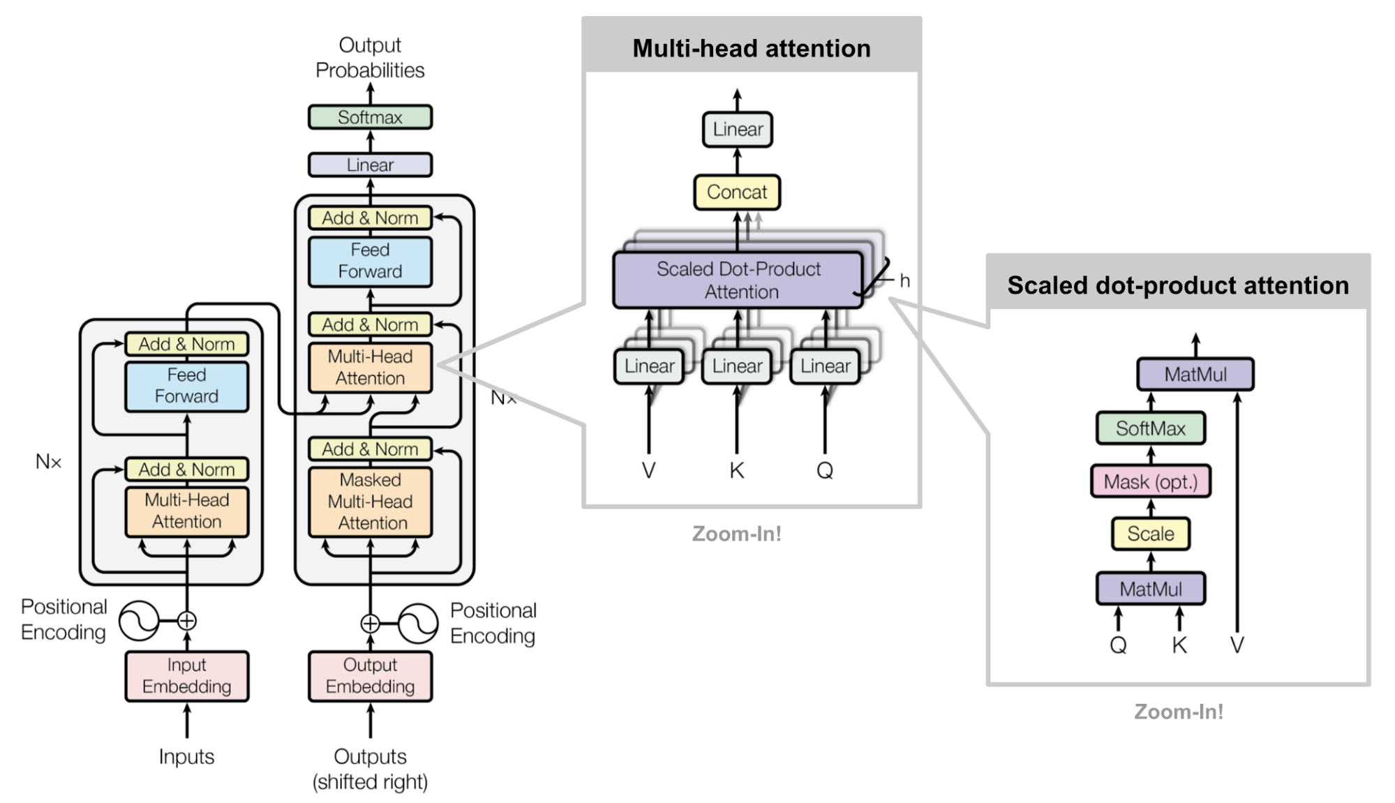
• The Encoder Stack: Its job is to process the entire input sequence (e.g., an audio spectrogram or a sentence) and build a rich, context-aware representation of it.
• The Decoder Stack: Its job is to generate the output sequence (e.g., a transcript) one element at a time. It uses the encoder's representation to inform its generation process.

Unlike earlier models that used RNNs for the encoder and decoder, the Transformer uses stacks of identical layers built around self-attention. The original paper used a stack of 6 encoder layers and 6 decoder layers.

Let's start by looking at the components that make up a single encoder layer.

2. Building an Encoder Layer

An encoder layer must process a sequence of input vectors and produce a sequence of output vectors of the same dimension, incorporating contextual information. It does this using four key components.

2.1. Positional Encoding

As we discussed, the self-attention mechanism is permutation-invariant. To give the model information about the order of the sequence, we inject a "positional encoding" vector into each input embedding.

These vectors are not learned; they are calculated using a clever function involving sine and cosine waves of different frequencies.

Where:

• pos is the position of the token in the sequence.
• i is the dimension within the embedding vector.
• $d_{\text{model}}$ is the dimension of the embedding (e.g., 512).

The intuition here is that for any fixed offset $k$, $P{E}_{pos+k}$ can be represented as a linear function of $P{E}_{pos}$. This property is thought to make it easy for the model to learn to attend to relative positions. The positional encoding vector is simply added to the input embedding.

2.2. Multi-Head Attention

In the last lesson, we learned about single-head self-attention. The Transformer improves on this with Multi-Head Attention. Instead of calculating attention once, it does it multiple times in parallel.

This has two main benefits:

1. Focus on Different Relationships: It allows the model to jointly attend to information from different "representation subspaces." For example, one attention head might learn to track syntactic dependencies, while another tracks semantic relationships.
2. Expanded Focus: It helps the model focus on multiple relevant words at once. In the sentence, "The animal didn't cross the street because it was too tired," one head might learn for "it" to attend to "animal," while another head learns for "it" to attend to "tired."

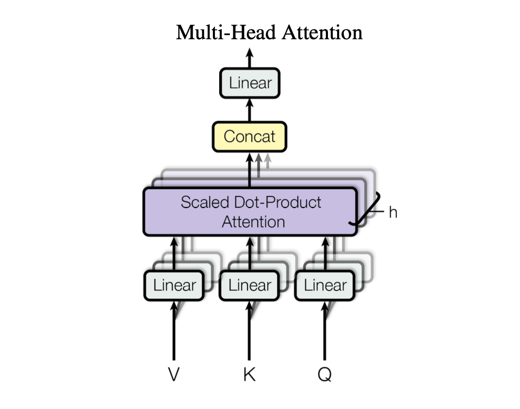
The mechanism works as follows:

1. Projection: The input vectors (or the Q, K, V matrices) are not fed into one attention function. Instead, they are linearly projected $h$ times (where $h$ is the number of heads) using different, learned weight matrices ($W_i^Q,W_i^K,W_i^V$ for each head $i$). This creates $h$ sets of queries, keys, and values.
2. Parallel Attention: Scaled dot-product attention is applied in parallel to each of these projected sets, yielding $h$ output matrices.
3. Concatenation & Final Projection: The $h$ output matrices are concatenated and then projected back to the original model dimension with another learned weight matrix, $W^O$.

2.3. Position-wise Feed-Forward Network (FFN)

After the multi-head attention sub-layer, the output for each position is passed through an identical but separate Feed-Forward Network (FFN). This component adds further processing capacity and non-linearity.

It consists of two linear transformations with a ReLU activation in between:
$\mathrm{FFN}(x)=\max (0,xW\_1+b\_1)W\_2+b\_2$

• The input and output dimensions are $d_{\text{model}}$.
• The inner-layer dimension is typically larger (e.g., $d_{ff}=4\times d_{\text{model}}$). For a 512-dimension model, this would be $512\to 2048\to 512$.

This network is called "position-wise" because it processes each position's vector independently.

2.4. Residuals and Layer Normalization

To make the network deep and stable, two more crucial elements are added. Each of the two sub-layers (Multi-Head Attention and FFN) in an encoder layer has a residual connection around it, followed by layer normalization.

The output of each sub-layer is calculated as: $\mathrm{LayerNorm}(x+\mathrm{Sublayer}(x))$.

• Residual Connection: This is the x + ... part, a concept from ResNets. It helps combat the vanishing gradient problem in deep networks and allows for easier information flow.
• Layer Normalization: This normalizes the outputs of the sub-layer, stabilizing the training dynamics. Unlike batch normalization, which normalizes across the batch, layer normalization normalizes across the features for each individual sequence.

With these four components, we can now define a full encoder layer.

3. Assembling the Decoder

The decoder's job is to generate the output sequence. It shares many components with the encoder, but with a few key differences to handle its generative, auto-regressive nature. A decoder layer has three sub-layers instead of two.

1. Masked Multi-Head Self-Attention: The decoder first performs self-attention on the output sequence it has generated so far. However, to maintain the auto-regressive property (i.e., the prediction for the current token can only depend on previous tokens), we must prevent it from "peeking ahead." This is done by applying a mask to the attention scores matrix before the softmax step. The mask sets the scores for all future positions to $-\infty$, which makes their softmax probabilities zero.

2. Encoder-Decoder Attention: This is where the decoder interacts with the encoder. This sub-layer is a multi-head attention mechanism, but with a twist:

   • The Queries (Q) come from the output of the previous decoder layer (the masked self-attention).
   • The Keys (K) and Values (V) come from the output of the final encoder layer.
     This allows every position in the decoder to attend to all positions in the input sequence, helping it decide which parts of the input are most relevant for generating the next output token.

3. Position-wise Feed-Forward Network: This is identical to the FFN in the encoder.

Like the encoder, each of these three sub-layers is also wrapped in a residual connection and followed by layer normalization.

4. The Full Picture: Training and Inference

To put it all together, let's trace the data flow during training.

To summarize the training process:

1. Encoder Pass: The entire source sequence is fed into the encoder stack. The output of the top encoder layer (the K and V matrices) is produced in one go.
2. Decoder Pass: The entire target sequence, shifted right by one position and prepended with a start-of-sequence token, is fed into the decoder stack.
3. Masked Self-Attention: The decoder uses masked self-attention to process the target sequence without looking ahead.
4. Encoder-Decoder Attention: At each decoder layer, the model uses the encoder's output (K and V) to cross-reference the source sequence.
5. Final Output Layer: The output from the top decoder layer is passed through a final linear layer (to project to the vocabulary size) and a softmax function to get the probability distribution over the next possible token.
6. Loss Calculation: The output probabilities are compared against the actual target sequence (the ground truth), and a loss (e.g., cross-entropy) is calculated to update the model's weights via backpropagation.

Crucially, all of this happens in a single, parallelizable forward pass, which is why Transformers are so efficient to train compared to RNNs.

5. From Theory to Code

Your background in computer science and experience with PyTorch will make it valuable to see how these theoretical blocks translate into code. While we will implement these components in later lessons, watching a guided implementation can solidify your understanding now.

Conclusion

In this lesson, we assembled the complete Transformer architecture from its fundamental building blocks. We've seen how it moves beyond the simple self-attention mechanism to create a deep, powerful, and highly parallelizable model for sequence-to-sequence tasks.

Key Takeaways:

• The Transformer consists of an encoder stack and a decoder stack.
• Positional Encodings are added to the input embeddings to provide the model with sequence order information.
• Multi-Head Attention allows the model to learn different types of relationships in parallel by using multiple sets of Q, K, V projections.
• Each layer contains Feed-Forward Networks for additional non-linear processing and is wrapped with residual connections and layer normalization for stable training.
• The decoder has three sub-layers: a masked self-attention layer to preserve auto-regression, an encoder-decoder attention layer to consult the input sequence, and an FFN.
• The entire model can be trained in a single, parallel forward-backward pass, a major advantage over recurrent models.

Preview of the Next Lesson:
Now that we have a solid theoretical and high-level code understanding of the Transformer's architecture, our next step is to get our hands dirty. In the next lesson, we will begin the practical implementation, starting with the core of the model: implementing a multi-head self-attention layer in PyTorch, including support for causal masking.