Visualizing High-Dimensional Data with t-SNE

Hello! Welcome to the next lesson in our journey through unsupervised learning.

Introduction

In our last lesson, we implemented Principal Component Analysis (PCA), a powerful linear technique for dimensionality reduction. We saw how it identifies the directions of maximum variance in the data and projects the data onto a lower-dimensional subspace. PCA is excellent for decorrelating features and reducing dimensionality for subsequent modeling tasks. However, its linearity means it can't capture complex, non-linear structures, like data lying on a curved manifold—think of a "swiss roll" shape.

Today, we will explore t-Distributed Stochastic Neighbor Embedding (t-SNE), a non-linear technique designed specifically for visualizing high-dimensional data. While PCA's goal is to preserve global variance, t-SNE's goal is to preserve local neighborhood structures. It tries to ensure that points that are close to each other in high-dimensional space remain close in the low-dimensional map (usually 2D or 3D).

This makes t-SNE incredibly effective at revealing the underlying cluster structures in a dataset, as you can see in the comparison below.

In this lesson, you'll learn how to apply t-SNE for high-dimensional data visualization. We'll cover the intuition behind the algorithm, its key mathematical components, and how to use it effectively in practice, including how to interpret its results and avoid common pitfalls.

1. The Core Idea: Keeping Neighbors Together

At its heart, t-SNE tries to solve an intuitive problem: how can we arrange points on a 2D map so that the arrangement reflects the "neighborliness" of those points in their original, high-dimensional space?

It does this through an iterative process of attraction and repulsion, a bit like a physics simulation.

The key takeaway is that t-SNE isn't just a simple projection like PCA. It's an optimization algorithm that actively arranges the points in the low-dimensional space to best reflect the local similarities of the original data. But how does it quantify these "similarities"? This is where probabilities come into play.

2. How t-SNE Works: The Algorithm

t-SNE evolved from an earlier algorithm called Stochastic Neighbor Embedding (SNE). Understanding the progression from SNE to t-SNE makes the entire process much clearer. The core of the algorithm involves two main stages:

1. Constructing a probability distribution over pairs of high-dimensional objects.
2. Defining a similar distribution for the low-dimensional points and minimizing the difference between the two.

Let's break this down with the help of a detailed video.

Mathematical Recap

Let's quickly formalize the key mathematical steps you just saw. Given your background, this structured view will help consolidate your understanding.

After working through these resources, you should have a solid grasp of both the intuitive goal and the mathematical machinery of t-SNE. You've essentially seen how it sets up an objective function (KL divergence) and optimizes the positions of points in the low-dimensional space using gradient descent, just like training a neural network.

Test your understanding!

The primary innovation of t-SNE over its predecessor SNE is the use of the Student's t-distribution in the low-dimensional space. Why is this specific choice so important? What problem does it solve and how?

Show answer

The Student's t-distribution is crucial because it solves the crowding problem. In high dimensions, there's a lot of "room," so points can have many neighbors at a moderate distance. When you try to map this to a low-dimensional space (like 2D), there isn't enough room to place all those moderate-distance neighbors around a central point without them getting "crowded."

The t-distribution has "heavier tails" than a Gaussian distribution. This means that points can be placed farther apart in the low-dimensional map and still have a relatively high similarity score ($q_{ij}$). This allows the model to create more space between clusters of points that are only moderately close in the high-dimensional space, leading to cleaner, more spread-out, and more interpretable visualizations.

3. Applying t-SNE with Scikit-learn

Now that we understand the theory, let's move to the practical application. Scikit-learn provides a robust and easy-to-use implementation of t-SNE.

Since you implemented PCA from scratch in the previous lesson, you'll appreciate how libraries like scikit-learn encapsulate complex algorithms. If you're curious, the t-SNE from Scratch article (resource LINK) provides a full NumPy implementation that mirrors the steps we've just discussed, but for this lesson, we'll focus on applying the sklearn version.

The most important hyperparameter is perplexity. It balances attention between local and global aspects of your data. Typical values are between 5 and 50. It's often recommended to try a few different values to see which one produces the most meaningful visualization for your specific dataset.

4. How to Interpret t-SNE Plots: Best Practices & Pitfalls

This is arguably the most important part of the lesson. t-SNE produces beautiful visualizations, but they can be easily misinterpreted.

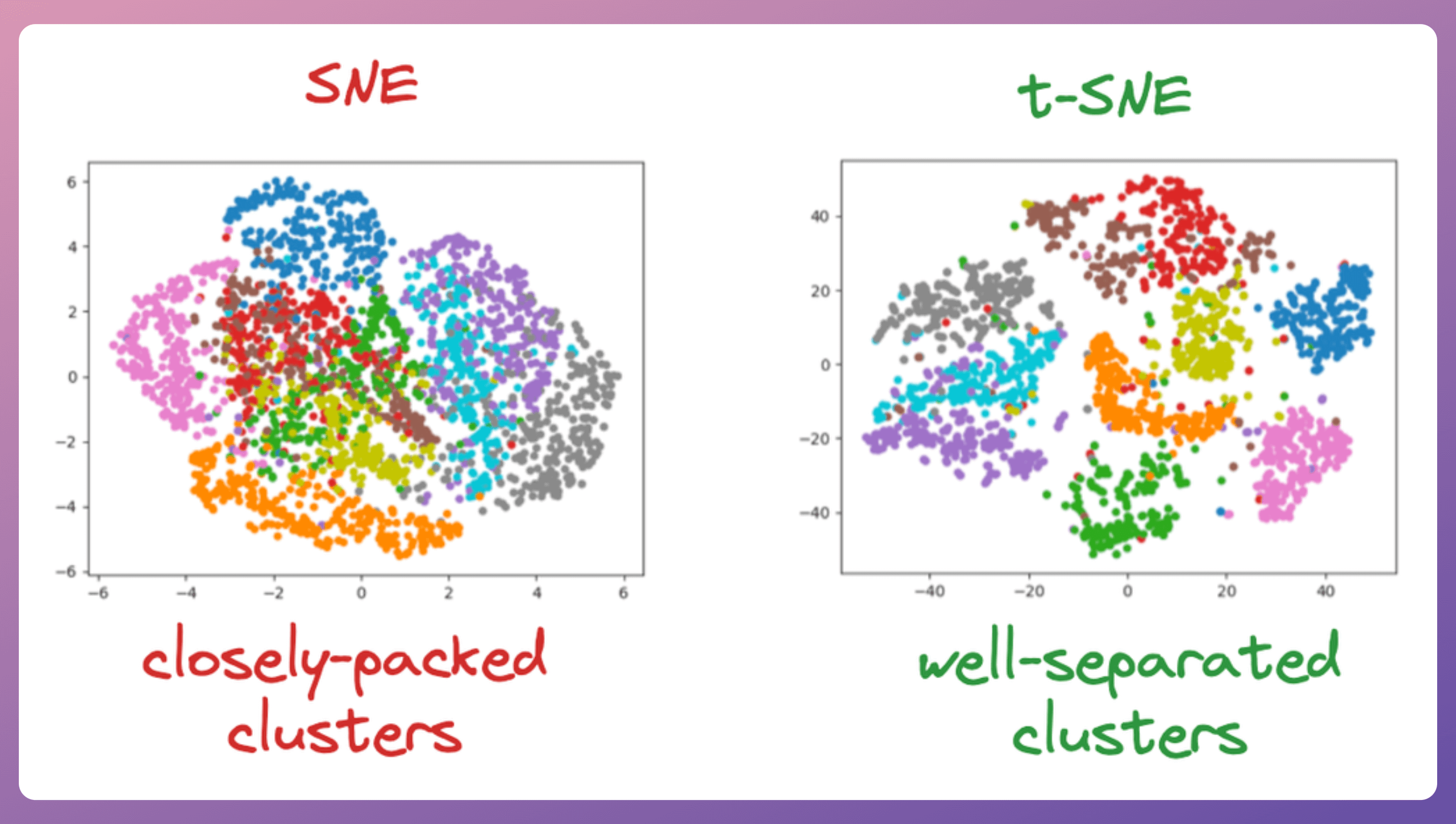
The visual separation is appealing, but you must be careful about the conclusions you draw.

Let's summarize the rules for interpreting t-SNE plots:

• DON'T interpret cluster sizes. The density of a cluster in a t-SNE plot is not meaningful. t-SNE will expand dense clusters and contract sparse ones to make their densities more uniform.
• DON'T interpret the distances between clusters. A large gap between two clusters doesn't necessarily mean they are "more different" than two clusters with a smaller gap. The global geometry is not preserved.
• DON'T use t-SNE for anything other than visualization/exploration. Unlike PCA, t-SNE is not a valid preprocessing step for other ML models. The algorithm is not designed to create a meaningful transformation for new data points.
• DO run the algorithm multiple times. The optimization process is stochastic (it involves random initialization). If the clusters you see are not stable across multiple runs, they are likely artifacts of the optimization.

Conclusion

In this lesson, we dove deep into t-SNE, a powerful non-linear technique for visualizing high-dimensional data. We moved from the high-level intuition to the underlying mathematical mechanics and practical application.

Key Takeaways:

• Purpose: t-SNE is a visualization tool that excels at revealing the local, non-linear structure of high-dimensional data, such as clusters.
• Mechanism: It works by modeling pairwise similarities as probability distributions in both the high-dimensional and low-dimensional spaces, and then uses gradient descent to minimize the KL divergence between them.
• Key Innovation: The use of a Student's t-distribution in the low-dimensional space solves the "crowding problem," allowing for cleaner separation between clusters.
• Hyperparameters: Perplexity is the most crucial hyperparameter, defining the effective number of neighbors for each point. Experimenting with it is key.
• Interpretation: Be cautious! Do not interpret cluster size or inter-cluster distances. The results are stochastic. Use t-SNE for exploration, not as a general-purpose dimensionality reduction tool for modeling.

Preview of the next lesson:
We've now looked at two dimensionality reduction techniques: PCA for linear data transformation and t-SNE for non-linear data visualization. Next, we will return to the task of formal clustering. We'll explore Gaussian Mixture Models (GMMs), a probabilistic approach that assumes data points are generated from a mixture of several Gaussian distributions. You'll learn how to implement GMMs using the powerful Expectation-Maximization (EM) algorithm, which provides a more formal and statistically grounded way to identify clusters compared to the visual exploration offered by t-SNE.