Implementing GMMs with EM

Hello! Let's dive into our final lesson in the "Unsupervised Learning and Representation" module.

Introduction

In our previous lessons, we explored dimensionality reduction with PCA and visualization with t-SNE. While t-SNE is fantastic for visually identifying potential clusters, it doesn't provide a formal model of the data's probability distribution. Today, we bridge that gap by exploring Gaussian Mixture Models (GMMs), a powerful probabilistic approach to clustering.

A GMM assumes that the data points are generated from a mixture of several Gaussian (normal) distributions, each with its own mean and covariance. This allows GMMs to perform "soft clustering," where each data point has a probability of belonging to each cluster, making it more flexible than "hard clustering" methods like K-Means, which assign each point to a single cluster.

To fit a GMM to the data, we'll use a cornerstone algorithm in machine learning called Expectation-Maximization (EM). The EM algorithm is an elegant iterative method for finding maximum likelihood estimates of parameters in statistical models that have latent, or hidden, variables.

By the end of this lesson, you will be able to implement a Gaussian Mixture Model using the Expectation-Maximization algorithm, solidifying your understanding of probabilistic modeling and latent variable optimization.

1. From Hard to Soft Clustering: The GMM Concept

Let's start by contrasting GMMs with a more familiar clustering algorithm, K-Means.

• K-Means assigns each data point to the single closest cluster center. This is a hard assignment.
• GMMs take a probabilistic view. They model the data as if it were generated from a mix of several Gaussian distributions. Instead of a hard assignment, a GMM provides a probability that a data point belongs to each of the component Gaussians. This is a soft assignment.

Imagine data that is not perfectly spherical or has varying densities. K-Means might struggle, but a GMM, by modeling clusters as ellipses (contours of Gaussian distributions) of different sizes and orientations, can capture the structure far more effectively.

The GMM as a Generative Model

Formally, a GMM is a probability density function expressed as a weighted sum of $k$ Gaussian components:

$p(\mathbf{x})={\sum }_{j=1}^k{\varphi }_j\mathcal{N}(\mathbf{x}|{\mathbf{\mu }}_j,{\Sigma }_j)$

Where:

• $k$ is the number of clusters (Gaussian components).
• ${\varphi }_j$ are the mixing coefficients (the weights of each Gaussian), with ${\sum }_{j=1}^k{\varphi }_j=1$. You can think of ${\varphi }_j$ as the probability of picking the $j$-th Gaussian.
• $\mathcal{N}(\mathbf{x}|{\mathbf{\mu }}_j,{\Sigma }_j)$ is the probability density of point $\mathbf{x}$ under the $j$-th Gaussian component, which has its own mean ${\mathbf{\mu }}_j$ and covariance matrix ${\Sigma }_j$.

The core challenge is: if we observe a set of data points ${\mathbf{x}}_i$, how do we find the best parameters $\Theta =\{{\varphi }_j,{\mathbf{\mu }}_j,{\Sigma }_j{\}}_{j=1}^k$? This is a maximum likelihood estimation problem. However, we have a "chicken-and-egg" problem because we don't know which Gaussian component generated each data point. This unknown component identity is a latent variable.

2. The Expectation-Maximization (EM) Algorithm

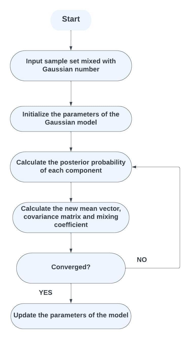
The EM algorithm is the iterative procedure we use to solve this problem of latent variables. It breaks the problem down into two repeating steps:

1. Expectation (E-step): Given our current estimates of the model parameters (${\varphi }_j,{\mathbf{\mu }}_j,{\Sigma }_j$), we calculate the probability that each data point ${\mathbf{x}}_i$ belongs to each cluster $j$. This is the "soft assignment" or "responsibility" of each cluster for each data point.
2. Maximization (M-step): Using these responsibilities as weights, we re-estimate the model parameters. We update the mean, covariance, and mixing coefficient for each cluster to better fit the data points that have been assigned to it.

We then repeat these E and M steps until the parameters converge.

Let's watch a more detailed explanation of how these steps work intuitively.

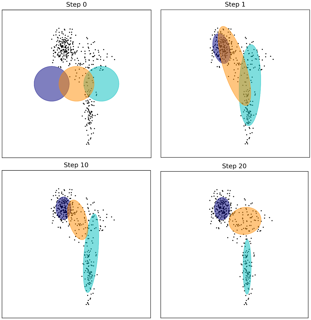
The iterative refinement process is beautifully illustrated by how the Gaussian components gradually move and reshape themselves to fit the data clusters.

3. The Mathematics of EM for GMMs

Now let's formalize the E and M steps with their update equations. Given your CS background and the course's goal of in-depth understanding, we'll first look at the what (the equations) and then the why (the derivation).

The Update Equations

Let's define $\gamma (z_{ij})$ as the "responsibility" that component $j$ takes for explaining data point ${\mathbf{x}}_i$.

E-Step: We calculate the responsibility for each point-cluster pair using our current parameters ${\Theta }_{\text{old}}=\{{\varphi }_j,{\mathbf{\mu }}_j,{\Sigma }_j\}$. This is essentially applying Bayes' theorem:

$\gamma (z_{ij})=\frac{{\varphi }_j\mathcal{N}({\mathbf{x}}_i|{\mathbf{\mu }}_j,{\Sigma }_j)}{{\sum }_{l=1}^k{\varphi }_l\mathcal{N}({\mathbf{x}}_i|{\mathbf{\mu }}_l,{\Sigma }_l)}$

The numerator is the "likelihood" of the point under Gaussian $j$ scaled by the "prior" probability of that Gaussian. The denominator is the total probability of the point under the whole mixture model, which serves as a normalization constant.

M-Step: We use these responsibilities to calculate the new parameters ${\Theta }_{\text{new}}$. Let $N_j={\sum }_{i=1}^n\gamma (z_{ij})$ be the effective number of points assigned to cluster $j$.

1. Update mixing coefficients: The new weight for a cluster is the average responsibility it takes for all data points.
   ${\varphi }_j^{\text{new}}=\frac{N_j}{n}$
   where $n$ is the total number of data points.

2. Update means: The new mean of a cluster is a weighted average of all data points, where the weights are the responsibilities.
   ${\mathbf{\mu }}_j^{\text{new}}=\frac{1}{N_j}{\sum }_{i=1}^n\gamma (z_{ij}){\mathbf{x}}_i$

3. Update covariances: The new covariance matrix is a weighted average of the outer products of the centered data points.
   ${\Sigma }_j^{\text{new}}=\frac{1}{N_j}{\sum }_{i=1}^n\gamma (z_{ij})({\mathbf{x}}_i-{\mathbf{\mu }}_j^{\text{new}})({\mathbf{x}}_i-{\mathbf{\mu }}_j^{\text{new}}{)}^T$

Why does EM work? (The Derivation)

You might be asking: why does this two-step process guarantee that we are maximizing the log-likelihood of our data? It's a non-obvious and elegant result based on a principle called the Evidence Lower Bound (ELBO).

The derivation is mathematically involved, but the core idea is exactly what's needed for a deep understanding of many advanced AI models (like Variational Autoencoders, which we'll see later). Given your goals, this is a crucial concept.

This process of coordinate ascent—first fixing parameters to optimize the bound's shape (E-step), then fixing the bound's shape to optimize the parameters (M-step)—guarantees convergence to a local maximum of the log-likelihood.

Test your understanding!

In the derivation of the EM algorithm, Jensen's inequality is used to transform the tricky $\log (\sum (\dots ))$ into a more manageable $\sum (\log (\dots ))$ by establishing a lower bound. What specific condition must be met for this lower bound to be "tight," meaning it is exactly equal to the true log-likelihood at the current parameter settings? How does the E-step ensure this condition is met?

Show answer

For the lower bound to be tight, the inequality in Jensen's theorem ($f(E[X])\ge E[f(X)]$ for a concave function $f$) must become an equality. This happens only if the random variable inside the expectation is a constant.

In the context of the EM derivation, the random variable is $\frac{P(x_i,z_i|\theta )}{Q(z_i)}$. For this to be constant for all values of the latent variable $z_i$, the distribution $Q(z_i)$ must be proportional to $P(x_i,z_i|\theta )$.

The E-step ensures this by setting $Q(z_i)$ to be exactly the posterior probability $P(z_i|x_i,\theta )$, which is defined as $\frac{P(x_i,z_i|\theta )}{P(x_i|\theta )}$. Since $P(x_i|\theta )$ is constant with respect to $z_i$, this choice makes $Q(z_i)$ proportional to $P(x_i,z_i|\theta )$, satisfying the condition for a tight bound.

4. Implementation from Scratch

With a solid grasp of the theory, we can now translate the EM algorithm for GMMs into code. Given your proficiency in Python and interest in fundamentals, implementing this from scratch is the best way to solidify your knowledge.

We will use a clear, object-oriented approach. The implementation will mirror the update equations we've just discussed.

This implementation gives you a fully functional GMM. You can see that once the mathematical steps are clear, the code becomes a direct translation. For a software engineer, it's also interesting to note how these operations can be vectorized using NumPy for efficiency, as shown in the em_gmm_vect function in the Duke University resource (LINK, section 6), which you can explore for further insight.

Conclusion

In this lesson, we have moved from simple clustering to a sophisticated probabilistic model. We dissected Gaussian Mixture Models and implemented the powerful Expectation-Maximization algorithm to fit them.

Key Takeaways:

• GMMs provide a flexible, probabilistic "soft clustering" by modeling data as a mixture of multiple Gaussian distributions.
• EM Algorithm is the key to training GMMs. It's an iterative two-step process for finding maximum likelihood estimates in models with latent variables.
• The E-Step calculates the responsibilities—the probability of each data point belonging to each cluster, given the current model.
• The M-Step updates the model parameters (means, covariances, mixing weights) using the responsibilities as weights.
• The magic of EM lies in its guarantee to increase the data log-likelihood at each iteration by maximizing a tight lower bound (ELBO).

This lesson concludes our module on Unsupervised Learning. You have now worked with linear dimensionality reduction (PCA), non-linear visualization (t-SNE), and probabilistic clustering (GMMs), giving you a robust toolkit for exploring and understanding the structure of unlabeled data.

Preview of the next lesson:
We are now ready to pivot to the core of modern AI: Deep Learning. In our next module, "Deep Neural Network Fundamentals," we will start from the ground up by building our first neural network, the Multi-Layer Perceptron (MLP). You will learn how information flows through the network in forward propagation to make a prediction. This will be the first step in our journey toward understanding and building complex deep learning architectures.