Implementing PCA from Scratch

Hello! Welcome back to our course.

Introduction

In our last lesson, we explored hierarchical clustering, a method for discovering nested group structures in data. We concluded by noting the challenge of working with high-dimensional datasets, often called the "curse of dimensionality," where having too many features can obscure patterns and make computation intractable.

Today, we'll tackle this problem head-on by studying Principal Component Analysis (PCA). PCA is a cornerstone of unsupervised learning and one of the most widely used techniques for dimensionality reduction. Its goal is not to group data points, but to find a more efficient way to represent the data by transforming the features themselves.

Essentially, PCA rotates the dataset into a new coordinate system where the axes (called principal components) are aligned with the directions of maximum variance. By keeping only the most important axes, we can reduce the number of dimensions while losing minimal information.

Dimensionality Reduction & Principal Component Analysis Illustration — This image illustrates the core idea of PCA: projecting data from a higher-dimensional space (3D) onto a lower-dimensional subspace (a 2D plane) that captures the most significant variation in the data.

In this lesson, you will learn to implement Principal Component Analysis (PCA) from scratch for dimensionality reduction. Given your background in computer science and mathematics, we will dive into the linear algebra that underpins the algorithm and translate it directly into a Python implementation.

1. The Mathematical Foundation of PCA

The central idea of PCA is to find a new set of orthogonal axes that best represents the data. "Best" in this context means capturing the maximum possible variance. The first principal component is the direction in the data with the largest variance. The second is the orthogonal direction with the next largest variance, and so on.

These directions are found by analyzing the covariance matrix of the data. As you may recall from your earlier studies, the covariance matrix describes how different variables in a dataset change together. The eigenvectors of this matrix point in the directions of maximum variance, and the corresponding eigenvalues indicate the magnitude of that variance.

This is the key insight:

Eigenvectors of the covariance matrix are the Principal Components.
Eigenvalues represent the amount of variance captured by each principal component.

Let's walk through the mathematical steps with a clear, simple example.

PCA : the math - step-by-step with a simple example

The video "PCA : the math - step-by-step with a simple example" by TileStats provides an excellent, detailed walkthrough of the calculations involved in PCA for a simple 2D dataset. It will solidify your understanding of the core mathematical operations.

Please watch from 01:13 to 14:56. The video covers the entire process: Steps Overview (01:13): Outlines the main steps of PCA. Data Centering (01:51): Subtracting the mean from each feature. Covariance Matrix (03:23): Calculating the covariance matrix from the centered data. Eigenvalues & Eigenvectors (05:23): Finding the eigenvalues and eigenvectors of the covariance matrix. Ordering & Transformation (09:53): Sorting the eigenvectors by their eigenvalues and using them to transform the data. Variance Analysis (12:45): Showing how the variance of the new components corresponds to the eigenvalues.

This video demonstrates that PCA is fundamentally an eigenvalue problem. By solving for the eigenvectors of the covariance matrix, we find the precise directions that capture the most information about our data's structure.

2. The PCA Algorithm: A Step-by-Step Guide

Now, let's formalize the steps required to perform PCA. We can think of it as a clear, sequential algorithm, which we will later implement in code.

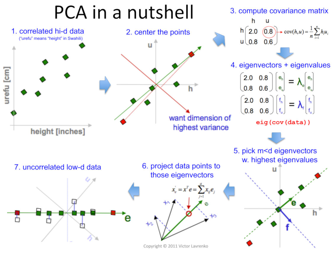
PCA in a Nutshell: A Step-by-Step Visual Guide — This infographic provides a concise visual summary of the PCA workflow, from data centering to the final projection.

The steps are:

Standardize the Data: Ensure all features are on a comparable scale. This is crucial because PCA is sensitive to the variance of the initial variables. We typically transform the data to have a mean of 0 and a standard deviation of 1.
Compute the Covariance Matrix: Calculate the covariance matrix for the standardized data. If our data matrix $X$ has $n$ samples and $d$ features, the covariance matrix $Σ$ will be a $d \times d$ matrix. For mean-centered data $X_{c}$ , this is $Σ = \frac{1}{n - 1} X_{c}^{T} X_{c}$ .
Calculate Eigenvalues and Eigenvectors: Decompose the covariance matrix to find its eigenvalues ( $λ_{i}$ ) and corresponding eigenvectors ( $v_{i}$ ).
Sort Eigenvectors: Sort the eigenvectors in descending order based on the magnitude of their corresponding eigenvalues. The eigenvector with the largest eigenvalue is the first principal component (PC1), the second largest corresponds to PC2, and so on.
Select Principal Components: Choose the top $k$ eigenvectors to form a new $d \times k$ matrix of principal components, $W$ . The value of $k$ determines the new dimensionality of your data.
Project the Data: Transform the original standardized data $X$ into the new $k$ -dimensional subspace by taking the dot product with the matrix of principal components: $X_{p ro j} = X \cdot W$ .

3. Implementing PCA from Scratch

With the theory and algorithm laid out, we can now translate these steps into Python code. We'll use NumPy for the numerical operations. Your experience with Python and linear algebra will be very useful here.

We will use a hands-on tutorial from Neuromatch Academy, which breaks the implementation into manageable coding exercises.

Tutorial 2: Principal Component Analysis

The Neuromatch tutorial "Principal Component Analysis" will guide you through implementing each part of the PCA algorithm. You will write the code to compute the covariance matrix, find the eigenvectors, and project the data.

Please work through the following sections and complete the coding exercises: Section 1: Calculate the eigenvectors of the sample covariance matrix. Read this section and complete Coding Exercise 1.1 (to implement get_sample_cov_matrix) and Coding Exercise 1.2 (to find and sort the eigenvectors). Section 2: Perform PCA by projecting data onto the eigenvectors. Read this section and complete Coding Exercise 2 (to build the full pca function). These exercises will have you build the core components of PCA step-by-step.

After completing these exercises, you will have a fully functional PCA implementation. You can see an alternative implementation in a class-based structure, which is common in machine learning libraries like scikit-learn.

How to implement PCA (Principal Component Analysis) from scratch with Python

To see these same steps assembled into a reusable Python class, watch this video from AssemblyAI. This will connect our from-scratch implementation to common software engineering patterns.

Watch the coding part of the video from 04:44 to 12:03. Notice how the logic is split between a fit method (calculating mean, covariance, and components) and a transform method (projecting the data).

Test your understanding!

In the fit method of the PCA class (from the AssemblyAI video), the data X is first mean-centered (X = X - self.mean), and then passed to np.cov(X.T). The documentation for np.cov states that it automatically subtracts the mean.

Why is it still necessary or good practice to perform the mean-centering step explicitly before calling np.cov?

Show answer

The explicit mean-centering is crucial for the transform method. The PCA model is "fit" on the training data, which involves calculating the mean and the principal components from that data. When you want to transform new, unseen data (or even the original training data), you must apply the exact same transformation. This includes subtracting the mean of the original training data before projecting it onto the principal components.

By calculating and storing self.mean during the fit phase, the transform method can correctly center any new data using the statistics of the training set. If the mean subtraction were only done implicitly inside np.cov, the transform method wouldn't have access to this crucial parameter.

4. Choosing the Number of Components

So far, we've transformed our data but haven't actually reduced its dimensionality. How do you decide how many principal components ( $k$ ) to keep?

The answer lies in the eigenvalues. Since each eigenvalue represents the variance captured by its corresponding eigenvector, we can calculate the proportion of total variance explained by each component.

The explained variance ratio for the $i$ -th component is:
$Explained Variance Ratio_{i} = \frac{λ _{i}}{\sum _{j = 1}^{d} λ _{j}}$
where $d$ is the original number of dimensions.

By plotting the cumulative explained variance (the sum of the explained variance ratios of the top $k$ components), we can choose a $k$ that retains a desired amount of the original information, such as 95% or 99% of the total variance.

Tutorial 2: Principal Component Analysis

The Neuromatch tutorial includes a great interactive demo to explore this concept.

Return to the tutorial and run Interactive Demo 2: Exploration of the correlation coefficient. Use the slider to change the correlation in the data and observe: How the eigenvalues (plotted in the "scree plot") change. When correlation is zero, the eigenvalues are nearly equal. The variance is spread evenly. As correlation approaches 1 or -1, one eigenvalue becomes much larger, indicating that most of the variance can be captured by a single principal component.

This trade-off is fundamental to dimensionality reduction: we sacrifice a small amount of variance (information) for a significant reduction in model complexity and computational cost.

Conclusion

In this lesson, we demystified Principal Component Analysis, breaking it down from a high-level concept into a concrete, step-by-step algorithm that you implemented from scratch.

Key Takeaways:

PCA is an unsupervised dimensionality reduction technique that transforms data into a new orthogonal basis of principal components.
These components are the eigenvectors of the data's covariance matrix, and they are ordered by their corresponding eigenvalues, which represent the variance captured along each axis.
The implementation workflow is: Standardize -> Compute Covariance Matrix -> Find Eigenvectors/Eigenvalues -> Sort -> Project.
The number of components to keep, $k$ , is chosen based on the desired cumulative explained variance, creating a trade-off between information retention and dimensionality.

Preview of the next lesson:
PCA is a powerful linear method, meaning it finds a flat subspace (like a line or a plane) to project the data onto. However, many high-dimensional datasets have complex, non-linear structures that look more like swiss rolls or intertwined manifolds. In our next lesson, we will explore t-Distributed Stochastic Neighbor Embedding (t-SNE), a non-linear technique specifically designed for visualizing such intricate high-dimensional data in 2D or 3D.