Tensor Parallelism: Sharding Weights for Parallel Layer Execution

Introduction

Welcome back! In our previous lesson, you successfully established a communication fabric between multiple GPUs by initializing a PyTorch distributed process group. You confirmed that your GPUs can "talk" to each other using the all_reduce collective operation. This is the foundational skill for any multi-GPU workload.

Now, we face the next major challenge in serving very large language models: what happens when even a single layer of a model, with its massive weight matrices, is too large to fit into one GPU's VRAM? This is a common problem with models like Llama 3 70B, where individual linear layers can be tens of gigabytes.

This is where Tensor Parallelism comes in. It is a model parallelism technique that shards individual tensors—specifically, the weight matrices of the model's layers—across multiple GPUs. This allows us to run a single layer's computation in parallel.

In this lesson, you will learn to explain tensor parallelism and how it shards weight matrices across GPUs to run a single layer in parallel. We will dissect the strategy pioneered by the Megatron-LM paper, focusing on how to parallelize the two workhorses of a transformer block: the MLP and the attention layers.

1. The Core Idea: Intra-Layer Parallelism

Before diving into the specifics of transformers, let's distinguish tensor parallelism from other strategies. In pipeline parallelism, you assign entire layers to different GPUs (inter-layer). In tensor parallelism, you split the computation within a single layer (intra-layer).

To build your intuition, let's watch a brief segment that contrasts these two approaches.

The key idea behind tensor parallelism is to break down large matrix multiplications. Consider a single linear layer defined by the operation $Y=XA$, where $X$ is the input activation and $A$ is the weight matrix.

There are two fundamental ways to parallelize this multiplication across two GPUs:

• Column-wise Parallelism: We split the weight matrix $A$ along its columns: $A=[A_1,A_2]$. The computation becomes $Y=X[A_1,A_2]=[X{A}_1,X{A}_2]$.

  • GPU 1 computes $Y_1=X{A}_1$.
  • GPU 2 computes $Y_2=X{A}_2$.
  • The input $X$ is replicated on both GPUs, and the output $Y$ is now sharded into $[Y_1,Y_2]$. This forward pass requires no communication between the GPUs.

• Row-wise Parallelism: We split the weight matrix $A$ along its rows: $A=\left[\begin{array}{c}{A}_1\\ A_2\end{array}\right]$. To make the matrix dimensions compatible, we must also split the input $X$ along its columns: $X=[X_1,X_2]$. The computation becomes $Y=[X_1,X_2]\left[\begin{array}{c}{A}_1\\ A_2\end{array}\right]=X_1{A}_1+X_2{A}_2$.

  • GPU 1 computes a partial result $Y_{p1}=X_1{A}_1$.
  • GPU 2 computes another partial result $Y_{p2}=X_2{A}_2$.
  • To get the final result $Y$, we must sum the partial results: $Y=Y_{p1}+Y_{p2}$. This requires an all-reduce communication step.

This distinction is crucial. The genius of the Megatron-LM approach is in combining these two sharding strategies to minimize communication.

2. Parallelizing the MLP Block

A standard transformer MLP (or feed-forward) block consists of two linear layers with a non-linear activation function (like GeLU) in between:

1. $Y=\text{GeLU}(XA)$
2. $Z=YB$

Here's how tensor parallelism is applied, step-by-step:

Step 1: First Linear Layer (Column-wise)

The first weight matrix, $A$, is sharded column-wise.

• The input activation $X$ is fully replicated on each GPU.
• Each GPU computes its part of the product: on GPU 1, it's $X{A}_1$; on GPU 2, it's $X{A}_2$.
• The result is a sharded activation, $[Y_1^{\prime },Y_2^{\prime }]$, where $Y_1^{\prime }=X{A}_1$ and $Y_2^{\prime }=X{A}_2$.

Step 2: Non-Linear Activation (GeLU)

Now, we apply the GeLU activation. Since GeLU is an element-wise function, it can be applied independently to each shard without any communication:

• GPU 1 computes $Y_1=\text{GeLU}(Y_1^{\prime })$.
• GPU 2 computes $Y_2=\text{GeLU}(Y_2^{\prime })$.
• The result is still a sharded activation, $[Y_1,Y_2]$.

This is a critical design choice. If we had used row-wise parallelism for the first layer, we would have partial results that would need to be all-reduced before the non-linearity could be applied correctly, as $\text{GeLU}(a+b)\ne \text{GeLU}(a)+\text{GeLU}(b)$. By using column-wise parallelism, we push the communication to a later stage.

Step 3: Second Linear Layer (Row-wise)

The second weight matrix, $B$, is sharded row-wise.

• The input to this layer, $Y$, is already sharded from the previous step.
• The matrix multiplication is now $Z=[Y_1,Y_2]\left[\begin{array}{c}{B}_1\\ B_2\end{array}\right]=Y_1{B}_1+Y_2{B}_2$.
• GPU 1 computes its partial result $Z_{p1}=Y_1{B}_1$.
• GPU 2 computes its partial result $Z_{p2}=Y_2{B}_2$.

Step 4: Final All-Reduce

To get the final, correct output $Z$, we must sum the partial results. This requires an all-reduce operation across the GPUs. After the all-reduce, each GPU holds the identical, complete tensor $Z$.

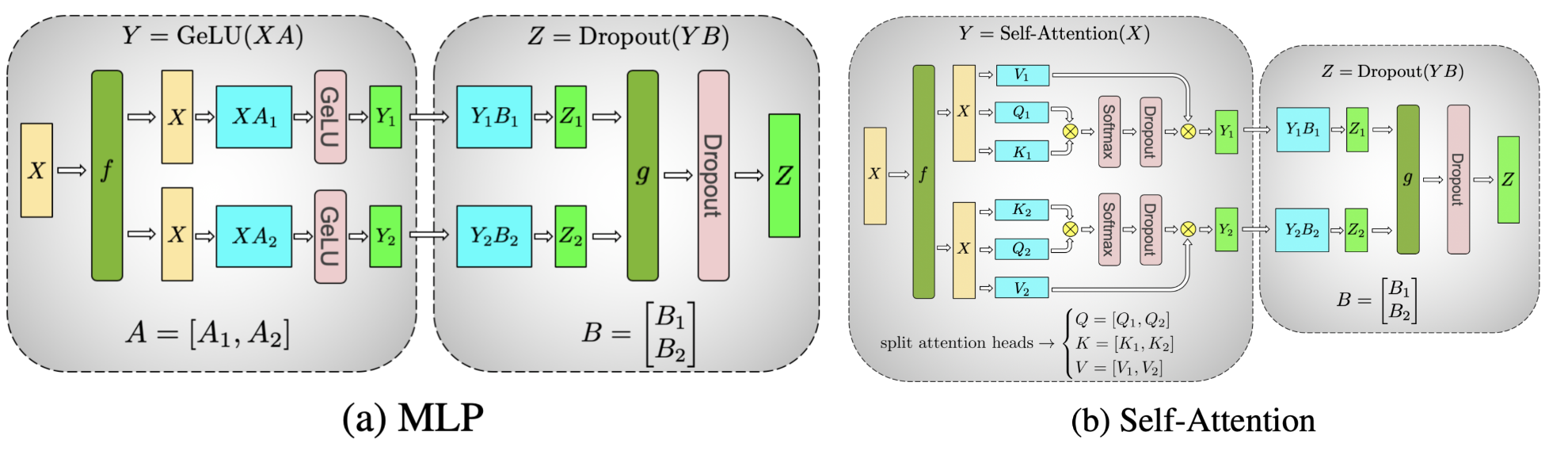
To get a much deeper understanding of this process, including the mathematical justification and excellent diagrams, please read the following post.

3. Parallelizing the Multi-Head Attention Block

The same principles apply to the Multi-Head Attention (MHA) block, which is even more naturally suited for this kind of parallelism because the computations for different attention heads are independent.

The MHA block performs these main operations:

1. Project input $X$ into Query, Key, and Value tensors: $Q=X{W}_Q$, $K=X{W}_K$, $V=X{W}_V$.
2. Split $Q,K,V$ into multiple heads.
3. Compute scaled dot-product attention for each head.
4. Concatenate head outputs and project with an output matrix: $Z=\text{Concat}(\text{heads})W_O$.

Here is the parallelization strategy:

Step 1: Q, K, V Projections (Column-wise)

The weight matrices for the query, key, and value projections ($W_Q,W_K,W_V$) are all sharded column-wise. This is equivalent to splitting the total number of attention heads across the available GPUs.

• The input $X$ is replicated on all GPUs.
• Each GPU computes the Q, K, and V projections for its assigned subset of heads. The results are sharded Q, K, and V tensors.

Step 2: Scaled Dot-Product Attention (Local)

Since each GPU has all the data it needs for its subset of heads, it can perform the entire scaled dot-product attention computation locally, without any communication.

Step 3: Output Projection (Row-wise)

The output projection matrix, $W_O$, is sharded row-wise.

• Each GPU takes its local attention output and multiplies it by its local shard of $W_O$.
• This produces a partial result for the final output tensor on each GPU.

Step 4: Final All-Reduce

Just like in the MLP block, an all-reduce operation is needed to sum the partial outputs from each GPU. The result is the complete, replicated output of the attention block.

Please return to the article from the previous section to see this logic applied to the attention layer.

4. Communication: The Systems-Level Cost

We've successfully parallelized a transformer block, but it comes at a cost: communication. For each transformer layer in the forward pass, we introduced two all-reduce operations: one at the end of the attention block and one at the end of the MLP block.

These collective operations are the primary overhead of tensor parallelism. Their performance is highly sensitive to the bandwidth and latency of the interconnects between GPUs.

• Intra-Node Communication: When GPUs are in the same server, they are often connected by a high-speed interconnect like NVLink, which offers bandwidth in the hundreds of GB/s.
• Inter-Node Communication: When GPUs are in different servers, they communicate over standard networking like Ethernet or InfiniBand, which is significantly slower.

Because of the frequent communication, tensor parallelism is most effective and almost exclusively used for GPUs within a single node. Trying to perform tensor parallelism across a slow network would lead to the communication time completely dominating the computation time, making the system highly inefficient.

The following talk provides a formal analysis of this trade-off.

Conclusion

In this lesson, you have deconstructed the concept of tensor parallelism and seen how it applies to the core components of a transformer. You've gone beyond a superficial understanding to see why specific sharding choices are made to minimize communication overhead. This mental model, balancing computation and communication, is fundamental to designing efficient distributed inference systems.

Key Takeaways:

• Tensor Parallelism (TP) is an intra-layer model parallelism technique that shards weight matrices and activations across multiple GPUs.
• The Megatron-LM strategy for an MLP block uses a column-wise split for the first linear layer and a row-wise split for the second. This strategically places a single all-reduce operation after the non-linearity.
• The attention block is parallelized by splitting the attention heads across GPUs. This involves a column-wise split for Q/K/V projections and a row-wise split for the output projection, also requiring one final all-reduce.
• A standard transformer layer requires two all-reduce operations in the forward pass.
• Due to this communication overhead, TP is most efficient when used with high-bandwidth, low-latency interconnects like NVLink, making it primarily an intra-node (within a single server) scaling strategy.

Preview of the Next Lesson:

Theory is essential, but as you requested, our focus is on practical implementation. In the next lesson, "Implement tensor-parallel inference for a transformer block," you will translate today's concepts into code. We will take a PyTorch transformer block, manually shard its weight matrices across two GPUs, and write the forward pass, complete with the necessary all_reduce calls to make it work.