Tensor-Parallel Transformer Inference

Introduction

Welcome back. In the previous lesson, we established a solid theoretical foundation for tensor parallelism. You learned how the Megatron-LM strategy uses a clever combination of column-wise and row-wise sharding to parallelize the matrix multiplications within a transformer block, minimizing communication by strategically placing all_reduce operations.

Today, we transition from theory to practice, directly addressing your goal of hands-on implementation. This lesson is designed to equip you with the modern tools to implement the concepts we just discussed. We will take a standard transformer block and use PyTorch's native tensor parallelism APIs to shard it across multiple GPUs. You will not only write the code but also verify its correctness, ensuring you understand how high-level abstractions map to the low-level operations we've studied.

By the end of this lesson, you will have implemented tensor-parallel inference for a transformer block, including the necessary communication steps, and verified that it produces the correct output.

1. From Manual Primitives to Modern Abstractions

In the last lesson, we visualized tensor parallelism as a sequence of operations: shard weights, perform local matrix multiplication, and then call all_reduce. While it's possible to implement this manually using raw torch.distributed primitives, this approach is verbose and error-prone.

Given your background, you'll appreciate that robust systems are built on well-designed abstractions. PyTorch provides exactly that for tensor parallelism through its torch.distributed.tensor.parallel module. The core components of this API are:

• DeviceMesh: An abstraction that represents a group of devices (GPUs) and their topology. This is more powerful than a simple process group, as it can represent multi-dimensional layouts (e.g., for hybrid data and tensor parallelism), though we'll use a simple 1D mesh today.
• DTensor (Distributed Tensor): A tensor-like object that is aware of its sharded nature. It logically represents a global tensor while physically storing only a local shard on each GPU. Operations on DTensors automatically trigger the necessary communication.
• parallelize_module: A high-level function that takes a standard nn.Module and a "parallelization plan," and automatically converts its parameters and buffers to DTensors, effectively sharding the module across the DeviceMesh.

Our task is to define the correct parallelization plan, which directly maps to the column-wise and row-wise sharding strategy we already know.

2. The Megatron-LM Strategy in PyTorch

Let's revisit the core strategy. For a pair of linear layers like in an MLP, $Z=\text{GeLU}(XA)B$, we apply column-wise parallelism to the first matrix $A$ and row-wise parallelism to the second matrix $B$.

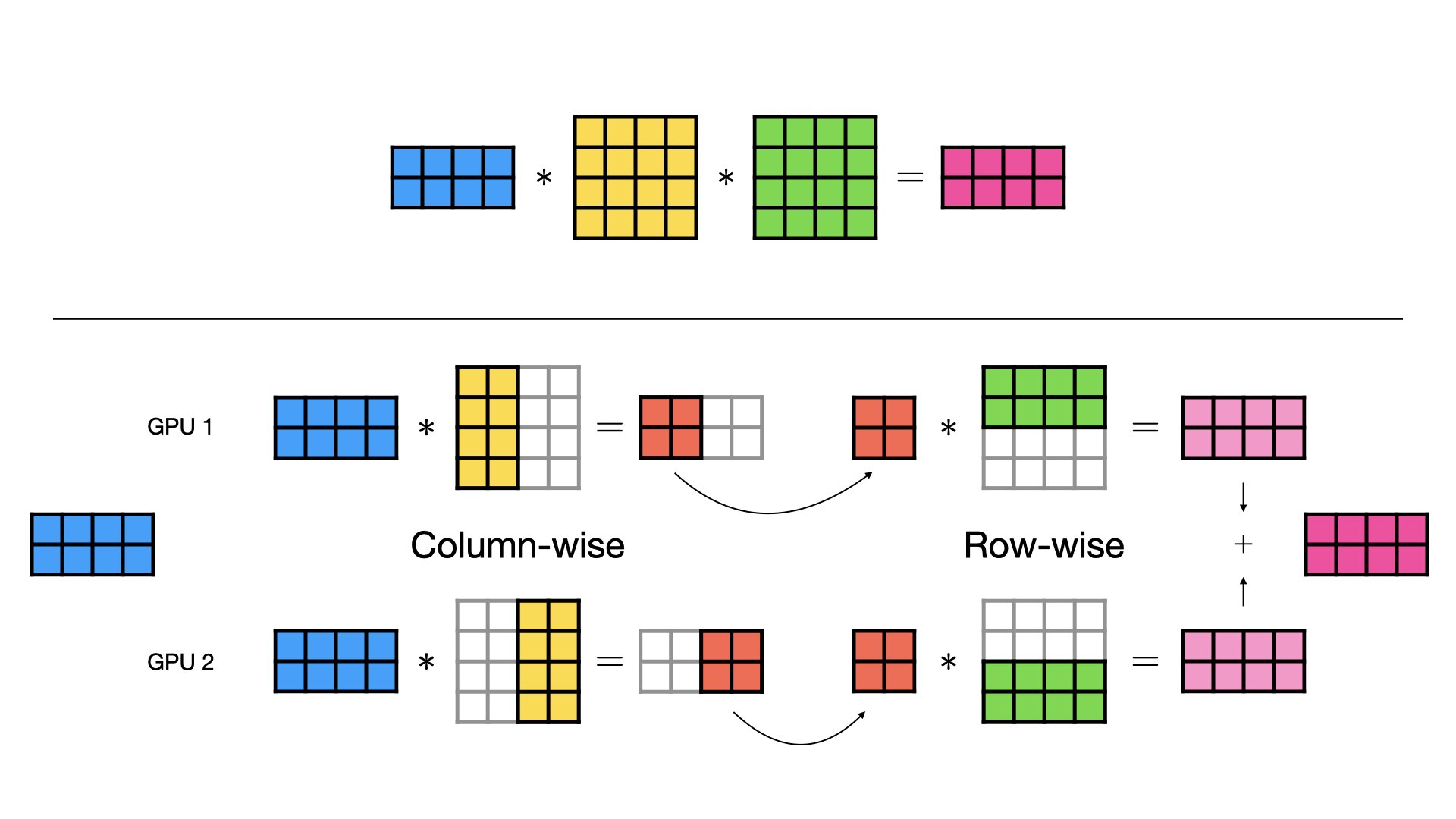
The torch.distributed.tensor.parallel API provides ParallelStyle objects to declare this intent:

• ColwiseParallel(): Use this for the first linear layer in a pair (e.g., w1 and w3 in a SwiGLU MLP, or the Q/K/V projections in attention). It shards the weight matrix along the column dimension.
• RowwiseParallel(): Use this for the second linear layer (e.g., w2 in the MLP, or the output projection wo in attention). It shards the weight matrix along the row dimension.

When you apply parallelize_module with a plan that has a RowwiseParallel layer following a ColwiseParallel layer, PyTorch understands that the input to the second layer is a sharded DTensor. It automatically performs the local matrix multiplication and then inserts the necessary all-reduce operation to produce the replicated output. This is the explicit "inclusion of the all-reduce communication step" that our learning outcome demands, handled cleanly by the API.

To see how these concepts are packaged in the PyTorch API, watch this short segment.

3. Implementing Tensor Parallelism for a Transformer Block

Now, let's get our hands dirty. We will apply this to a standard TransformerBlock. The process involves three main steps:

1. Set up the distributed environment and DeviceMesh.
2. Define the parallelize_plan for our TransformerBlock.
3. Apply the plan using parallelize_module.

The official PyTorch documentation provides an excellent tutorial that walks through this exact process for a Llama-style transformer block. Your main task for this lesson is to study and understand this implementation.

Dissecting the parallelize_plan

Let's break down the layer_tp_plan from the tutorial to connect it back to our theory.

For the FeedForward layer (a SwiGLU variant with w1, w2, w3):

• "feed_forward.w1": ColwiseParallel()
• "feed_forward.w3": ColwiseParallel()
  • The two initial projections are done in parallel. Their weights are sharded column-wise. The input x is replicated, and the outputs of w1(x) and w3(x) are sharded. The element-wise silu and multiplication can happen locally on the sharded data.
• "feed_forward.w2": RowwiseParallel()
  • The final projection's weight is sharded row-wise. It takes the sharded result from the previous step as input, performs a local matrix multiplication, and then an all_reduce is automatically executed to produce the final, replicated output of the MLP block.

For the Attention layer:

• "attention.wq": ColwiseParallel()
• "attention.wk": ColwiseParallel()
• "attention.wv": ColwiseParallel()
  • The Q, K, and V projection weights are sharded column-wise. This is equivalent to distributing the attention heads across the GPUs. The input is replicated, and the resulting Q, K, V tensors are sharded by the head dimension.
  • The scaled-dot-product attention can now be computed locally on each GPU for its subset of heads.
• "attention.wo": RowwiseParallel()
  • The output projection's weight is sharded row-wise. It takes the sharded attention output from the previous step, performs a local matmul, and again, triggers an all_reduce to produce the final, replicated output of the attention block.

This plan perfectly implements the two-all_reduce-per-layer strategy of Megatron-LM.

4. Code Exercise: A Verifiable Forward Pass

To solidify your understanding, let's write a self-contained script to perform a tensor-parallel forward pass. We won't run a full training loop; instead, we'll focus on verifying that the parallelized block produces the same output as a standard, single-GPU block.

Below is a Python script. Your task is to complete the tp_plan dictionary based on what you've just learned from the PyTorch tutorial.

Setup:
Save the following code as tp_forward_pass.py. You will need at least two GPUs to run this.

import os
import torch
import torch.nn as nn
import torch.distributed as dist
from torch.distributed.tensor.parallel import parallelize_module, ColwiseParallel, RowwiseParallel
from torch.distributed.device_mesh import init_device_mesh




# --- 1. Distributed Setup ---
def setup_distributed():
    dist.init_process_group("nccl")
    rank = dist.get_rank()
    world_size = dist.get_world_size()
    device = f"cuda:{rank}"
    torch.cuda.set_device(device)
    return rank, world_size, device




# --- 2. A Simple Transformer Block ---
class SimpleAttention(nn.Module):
    def __init__(self, hidden_size, num_heads):
        super().__init__()
        self.wq = nn.Linear(hidden_size, hidden_size)
        self.wk = nn.Linear(hidden_size, hidden_size)
        self.wv = nn.Linear(hidden_size, hidden_size)
        self.wo = nn.Linear(hidden_size, hidden_size)
        self.num_heads = num_heads
        self.head_dim = hidden_size // num_heads

    def forward(self, x):



        # In a real implementation, you'd reshape for multi-head attention
        # Here, we simplify to focus on the linear layers
        q = self.wq(x)
        k = self.wk(x)
        v = self.wv(x)



        # Simplified attention-like operation
        attn_output = q + k + v 
        return self.wo(attn_output)

class SimpleMLP(nn.Module):
    def __init__(self, hidden_size):
        super().__init__()
        self.w1 = nn.Linear(hidden_size, 4 * hidden_size)
        self.w2 = nn.Linear(4 * hidden_size, hidden_size)
        self.activation = nn.GELU()

    def forward(self, x):
        return self.w2(self.activation(self.w1(x)))

class TransformerBlock(nn.Module):
    def __init__(self, hidden_size, num_heads):
        super().__init__()
        self.attention = SimpleAttention(hidden_size, num_heads)
        self.mlp = SimpleMLP(hidden_size)

    def forward(self, x):



        # Simplified: no layer norms or residual connections
        x = self.attention(x)
        x = self.mlp(x)
        return x




# --- Main Execution ---
if __name__ == "__main__":
    rank, world_size, device = setup_distributed()

    if world_size < 2:
        print("This script requires at least 2 GPUs.")
        exit()




    # Hyperparameters
    batch_size = 4
    seq_len = 16
    hidden_size = 512
    num_heads = 8




    # --- 3. Create Models and Input ---
    # Create a reference model on the meta device
    with torch.device("meta"):
        model_ref = TransformerBlock(hidden_size, num_heads)




    # Instantiate the model to be parallelized on the meta device
    with torch.device("meta"):
        model_tp = TransformerBlock(hidden_size, num_heads)




    # Materialize the reference model on a single GPU (rank 0)
    model_ref.to_empty(device="cuda:0")
    model_ref.reset_parameters()




    # Materialize the TP model and load state from reference
    model_tp.to_empty(device=device)
    model_tp.load_state_dict(model_ref.state_dict())




    # --- 4. Define the Parallelization Plan ---
    # YOUR TASK: Complete this dictionary
    tp_plan = {



        # Attention block
        "attention.wq": ColwiseParallel(),
        "attention.wk": ColwiseParallel(),
        "attention.wv": ColwiseParallel(),
        "attention.wo": RowwiseParallel(),



        # MLP block
        "mlp.w1": ColwiseParallel(),
        "mlp.w2": RowwiseParallel(),
    }




    # --- 5. Apply Tensor Parallelism ---
    tp_mesh = init_device_mesh("cuda", (world_size,))
    model_tp = parallelize_module(model_tp, tp_mesh, tp_plan)




    # Create a random input tensor, replicated on all GPUs
    input_tensor = torch.rand(batch_size, seq_len, hidden_size, device=device)
    dist.broadcast(input_tensor, src=0) # Ensure all GPUs start with the same input




    # --- 6. Run Forward Passes and Compare ---
    # Run reference model on rank 0
    if rank == 0:
        output_ref = model_ref(input_tensor.to("cuda:0"))




    # Run TP model on all ranks
    output_tp = model_tp(input_tensor)




    # --- 7. Verification ---
    if rank == 0:



        # The output of the TP model should be replicated on all GPUs.
        # We compare the output from the TP model on rank 0 with the reference output.
        print("Comparing outputs...")
        are_close = torch.allclose(output_ref, output_tp.to("cuda:0"), atol=1e-5)
        print(f"Outputs are close: {are_close}")
        if not are_close:
            print("Difference:", torch.abs(output_ref - output_tp.to("cuda:0")).max())

    dist.destroy_process_group()

To run the script:
Use torchrun from your terminal. If you have 2 GPUs, it will automatically manage the processes.

torchrun --nproc_per_node=2 tp_forward_pass.py

When you run this, torchrun will launch two processes. Each process will initialize its own TransformerBlock, but the parallelize_module call will convert the linear layers into distributed modules. The weights of wq and w1 will be sharded column-wise, and the weights of wo and w2 will be sharded row-wise. The forward pass on model_tp will execute the two necessary all_reduce operations internally, and the final output will be a replicated tensor, identical on both GPUs and matching the output of the single-GPU reference model.

For another perspective on creating and applying the tp_plan, you can also consult this excellent third-party guide.

Conclusion

Congratulations! You have successfully bridged the gap from the theory of tensor parallelism to a concrete, working implementation. You've seen how modern PyTorch APIs provide powerful abstractions that map directly to the underlying sharding and communication strategies we studied. By defining a parallelize_plan, you instructed PyTorch to automatically shard weights and insert the critical all_reduce communication steps, and you verified that the distributed computation yields the correct result.

Key Takeaways:

• Modern tensor parallelism in PyTorch is implemented using abstractions like DeviceMesh, DTensor, and parallelize_module.
• A parallelize_plan is a dictionary that maps module names to ParallelStyle objects (ColwiseParallel, RowwiseParallel).
• This plan directly implements the Megatron-LM strategy: ColwiseParallel on the first linear layer(s) of a sub-component, and RowwiseParallel on the last.
• The RowwiseParallel style on a sharded input implicitly handles the all_reduce communication step, ensuring the output is correctly computed and replicated.
• By running a parallelized forward pass and comparing it to a reference, you can verify the correctness of your tensor-parallel implementation.

Preview of the Next Lesson:

Tensor parallelism is brilliant for scaling layers that are too big for one GPU, but it's not the only way to distribute a model. What if the entire model, even with TP, is still too large? Or what if we want to improve hardware utilization? In the next lesson, we will explore pipeline parallelism, where we partition the model between layers, assigning entire sequences of layers to different GPUs to work in an assembly-line fashion.