Introduction
Welcome back. In our previous lesson, you successfully implemented tensor parallelism, a technique for sharding individual model layers within a GPU cluster to handle massive weight matrices. You learned how to use PyTorch's parallelize_module to apply column-wise and row-wise sharding, effectively parallelizing the matrix multiplications inside attention and MLP blocks. This is known as intra-layer parallelism.
Today, we shift our focus to a complementary strategy: pipeline parallelism. Instead of splitting up individual layers, we will partition the model between layers, creating an assembly line where different GPUs are responsible for different sets of sequential layers. This is a form of inter-layer parallelism.
By the end of this lesson, you will be able to explain how pipeline parallelism partitions a model across multiple GPUs, understand the critical performance challenge it introduces—the "pipeline bubble"—and describe the primary technique used to overcome it. This conceptual foundation is essential before we move on to implementing it in the next lesson.
1. The Core Concept: A Model Assembly Line
At its heart, pipeline parallelism is an intuitive way to distribute a model that is too large to fit on a single GPU. You simply assign contiguous blocks of layers to different devices.
- Device 0 might handle layers 1-8.
- Device 1 might handle layers 9-16.
- Device 2 might handle layers 17-24.
- and so on.
During a forward pass, Device 0 processes the input and passes its output (the activations) to Device 1. Device 1 then performs its computations and passes its activations to Device 2. This continues until the final device computes the model's output. The backward pass works in reverse.
To get a clear visual and conceptual introduction to this idea, let's start with a section from the "LLMs from Scratch" guide.
LLMs from Scratch #007: Mastering Distributed Machine Learning ...
This article introduces model parallelism and clearly distinguishes pipeline parallelism from the tensor parallelism we covered previously. It frames pipeline parallelism as the conceptually simplest way to partition a model.
Read the section '7. Pipeline Parallelism', up to but not including 'The Layer-wise Parallelism Problem'. Focus on how it describes splitting parameters across GPUs by distributing layers and passing activations between them.
This video provides a similar explanation with a helpful hand-drawn diagram, contrasting the "inter-layer" splitting of pipeline parallelism with the "intra-layer" splitting of tensor parallelism you're already familiar with.
Ultimate Guide To Scaling ML Models - Megatron-LM | ZeRO | DeepSpeed | Mixed Precision
Watch this segment from Aleksa Gordić's video for a clear, visual explanation of how pipeline parallelism partitions a model's layers across different devices.
Watch from 7:35 to 9:27. Pay attention to how the presenter illustrates distributing blocks of transformer layers onto four separate devices.
2. The Inefficiency of Naive Pipelining: The Bubble
While conceptually simple, a naive implementation of pipeline parallelism is extremely inefficient. Consider a 4-GPU setup.
- Input data goes to GPU 0. GPUs 1, 2, and 3 are idle.
- GPU 0 finishes and sends activations to GPU 1. GPUs 0, 2, and 3 are idle.
- GPU 1 finishes and sends activations to GPU 2. GPUs 0, 1, and 3 are idle.
- GPU 2 finishes and sends activations to GPU 3. GPUs 0, 1, and 2 are idle.
This sequential dependency creates a significant amount of idle time on the GPUs, known as the pipeline bubble. In this naive setup, only one GPU is active at any given time, completely defeating the purpose of using multiple devices.
The following resources explain and visualize this problem perfectly.
LLMs from Scratch #007: Mastering Distributed Machine Learning ...
Let's return to the 'LLMs from Scratch' article to read about this critical inefficiency.
Read the subsection titled 'The Layer-wise Parallelism Problem'. It quantifies the terrible GPU utilization and sets the stage for the solution.
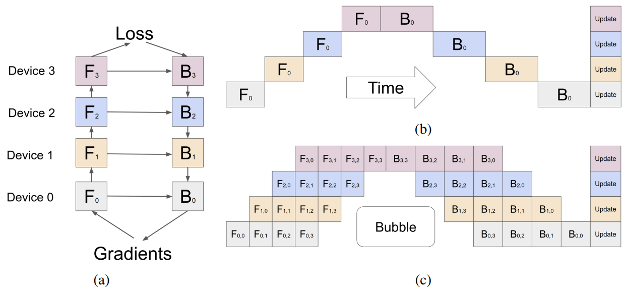
Now, see this inefficiency visualized. The diagram below, from NVIDIA, is a canonical representation of the pipeline parallelism process. Panel (b) shows the naive approach and the resulting idle time (the white "bubbles").
3. The Solution: Micro-batching and Scheduling
To mitigate the pipeline bubble, we don't process the entire input batch at once. Instead, we split the batch into smaller micro-batches. This allows the pipeline stages to operate in an overlapping, assembly-line fashion.
As soon as GPU 0 finishes processing the first micro-batch, it passes the activations to GPU 1. While GPU 1 works on micro-batch 1, GPU 0 can immediately start processing micro-batch 2. This overlapping of computation and communication "fills" the pipeline bubble and dramatically increases GPU utilization.
The following video provides an excellent explanation of this process.
Efficient Large-Scale Language Model Training on GPU Clusters Using Megatron-LM | Jared Casper
In this video, Jared Casper from NVIDIA explains how splitting a batch into micro-batches makes pipeline parallelism efficient. This directly corresponds to panel (c) in the diagram above.
Watch from 11:45 to 13:05. Focus on how the timeline diagram changes from the naive approach to one using micro-batches, filling the idle 'dark gray' spaces.
The efficiency of the pipeline is a function of the number of pipeline stages and the number of micro-batches. As a rule of thumb:
More micro-batches lead to a smaller bubble and higher efficiency. The way micro-batches are processed is determined by a pipeline schedule. Common schedules include:
- GPipe: A simple schedule where all forward passes for all micro-batches are executed first, followed by all backward passes. This is shown in the diagram above.
- 1F1B (One-Forward-One-Backward): A more advanced schedule that interleaves forward and backward passes to reduce the amount of activation memory that needs to be stored.
4. How to Partition a Model in PyTorch
Now that you understand the concept, let's briefly touch on how this partitioning is accomplished in code, which will be the focus of our next lesson. PyTorch's torch.distributed.pipelining API provides tools to achieve this.
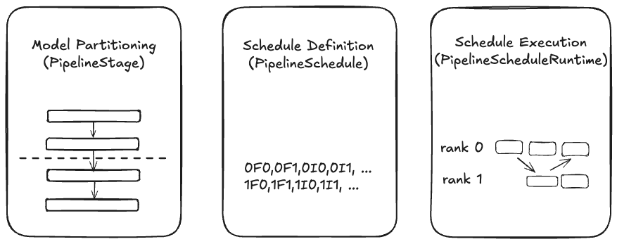
There are two primary ways to partition the model layers:
- Manual Partitioning: You explicitly define which layers belong to which GPU. For a model with 32 layers and 4 GPUs, you might manually assign layers 0-7 to rank 0, 8-15 to rank 1, and so on. This gives you full control but can be cumbersome.
- Tracer-based Splitting: You provide a
split_specthat tells a tracer where to "cut" the model graph. For example, you can specify that a split should occur aftermodel.layers[7]andmodel.layers[15]. The API then automatically handles the partitioning.
This tutorial from PyTorch provides the details. You don't need to dive deep into the code now, but skimming it will help you connect the concepts to the API we'll use next time.
Introduction to Distributed Pipeline Parallelism — PyTorch Tutorials ...
This official PyTorch tutorial demonstrates how to use the torch.distributed.pipelining API. Skim this section to see how partitioning is done in practice.
Read 'Step 1: Partition the Transformer Model'. Notice the two approaches: the manual mode where layers are deleted, and the tracer-based mode that uses a split_spec.
5. Tensor vs. Pipeline Parallelism: A System Design Choice
As an AI Systems Engineer, the crucial question is not just how to use these techniques, but when and why. Tensor and pipeline parallelism have distinct trade-offs.
| Feature | Tensor Parallelism (TP) | Pipeline Parallelism (PP) |
|---|---|---|
| Splits... | Within layers (intra-layer) | Between layers (inter-layer) |
| Communication | High overhead (all_reduce on weights) |
Lower overhead (point-to-point on activations) |
| Latency | Best on low-latency, high-bandwidth interconnect (NVLink) | More tolerant of higher-latency interconnect (Ethernet) |
| GPU Utilization | No bubble, generally high utilization | Suffers from a "bubble" (mitigated by micro-batching) |
| Typical Use Case | Within a node (e.g., across 8 GPUs in a server) | Across nodes (e.g., across multiple servers) |
This leads to a standard industry practice often called 3D Parallelism:
- Tensor Parallelism (1st Dimension): First, apply TP to make the model's layers fit within a single multi-GPU node. This is very efficient with fast interconnects like NVLink.
- Pipeline Parallelism (2nd Dimension): If the model is still too large after maxing out TP within a node (e.g., an 8-GPU node), apply PP across different nodes to distribute the remaining layers.
- Data Parallelism (3rd Dimension): Finally, use Data Parallelism to replicate this entire TP+PP setup and train on more data simultaneously, increasing throughput.
This article provides an excellent summary of these trade-offs and the resulting strategy.
LLMs from Scratch #007: Mastering Distributed Machine Learning ...
This final reading directly compares the two model parallelism techniques and explains how they are combined in practice to train enormous models.
Read the sections 'Tensor vs Pipeline Parallel Trade-offs' and '3D Parallelism Integration'. This synthesizes everything we've covered and provides the high-level system design perspective that is key to your goal.
Conclusion
In this lesson, we've established the conceptual framework for pipeline parallelism. You now understand how it differs from the tensor parallelism we previously studied and the critical role it plays in distributing truly massive models.
Key Takeaways:
- Pipeline parallelism (PP) is an inter-layer model parallelism strategy that partitions a model by assigning sequential blocks of layers to different GPUs.
- A naive implementation is highly inefficient due to the pipeline bubble, where most GPUs are idle while waiting for data from a previous stage.
- Micro-batching is the key technique to solve this, creating an assembly-line-like process that overlaps computation and communication to improve GPU utilization.
- PP has lower communication overhead than tensor parallelism and is better suited for communication across nodes (inter-node).
- In practice, a common strategy is to use Tensor Parallelism within nodes and Pipeline Parallelism across nodes.
Preview of the Next Lesson:
With this theoretical grounding, you are ready to get your hands on the code. In the next lesson, we will implement a forward pass for a pipeline-parallel model, where you will be responsible for managing micro-batches and the data transfers between stages using PyTorch's distributed APIs.