Introduction
In our last lesson, we focused on the primary performance challenge of pipeline parallelism: the pipeline bubble. You learned how to visualize this idle time on a GPU execution timeline and, more importantly, how to quantify its impact on compute utilization. We established that the bubble is fundamentally a compute utilization problem, driven by data dependencies between pipeline stages.
This lesson shifts our focus from compute to communication. While pipeline parallelism's main drawback is idle compute, tensor parallelism's primary challenge is its communication overhead. Your goal for this lesson is to analyze the communication overhead of tensor vs. pipeline parallelism, specifically comparing all-reduce and point-to-point operations.
By the end of this lesson, you will understand the distinct communication patterns of each strategy, their sensitivity to network hardware, and why production systems almost always use a hybrid approach to balance these trade-offs.
1. A Framework for Analyzing Communication Cost
Before diving into specific parallelism strategies, we need a formal model for communication cost. As a systems engineer, you'll often model performance before building, and communication is a critical component.
Any data transfer over a network, whether between GPUs in a server or across servers, has two primary costs:
- Latency (): A fixed, one-time cost to initiate the transfer. This is like the time it takes for a mail truck to start its engine and pull out of the depot, regardless of how much mail it's carrying.
- Bandwidth (): The rate at which data can be sent, measured in Gigabytes per second (GB/s). The time to transfer the data itself is the message size divided by the bandwidth. This is analogous to the speed of the mail truck on the highway.
These factors are captured in the simple but powerful alpha-beta model for the time () to send a message of size ():
where is the effective bandwidth achieved.
The physical hardware dramatically affects these values. Communication within a node over high-speed interconnects like NVIDIA's NVLink offers extremely low latency and very high bandwidth (e.g., 900 GB/s). Communication between nodes over technologies like InfiniBand or Ethernet has higher latency and lower bandwidth. This distinction is the single most important factor in designing distributed training and inference systems.
Let's ground these concepts in the common communication primitives used in PyTorch.
Communication Overhead Analysis
The article 'Communication Overhead Analysis' from ApX Machine Learning provides an excellent, concise overview of the key concepts. We will use it as a reference throughout this lesson.
Please read the sections 'Communication Primitives in Distributed Training' and 'Factors Influencing Communication Cost'. Focus on understanding the difference between collective operations like all_reduce and point-to-point operations like send/recv. Also, internalize the alpha-beta model and the list of factors that influence communication cost.
2. The Communication Pattern of Tensor Parallelism
Tensor Parallelism (TP) parallelizes computation within each layer. As you saw when implementing it, this involves sharding weight matrices. For example, in an MLP block, the first weight matrix is split column-wise.
After the distributed matrix multiplication X @ [A1, A2] = [X@A1, X@A2], each GPU holds a piece of the result. However, the next operation might require the complete result. This is where communication becomes necessary.
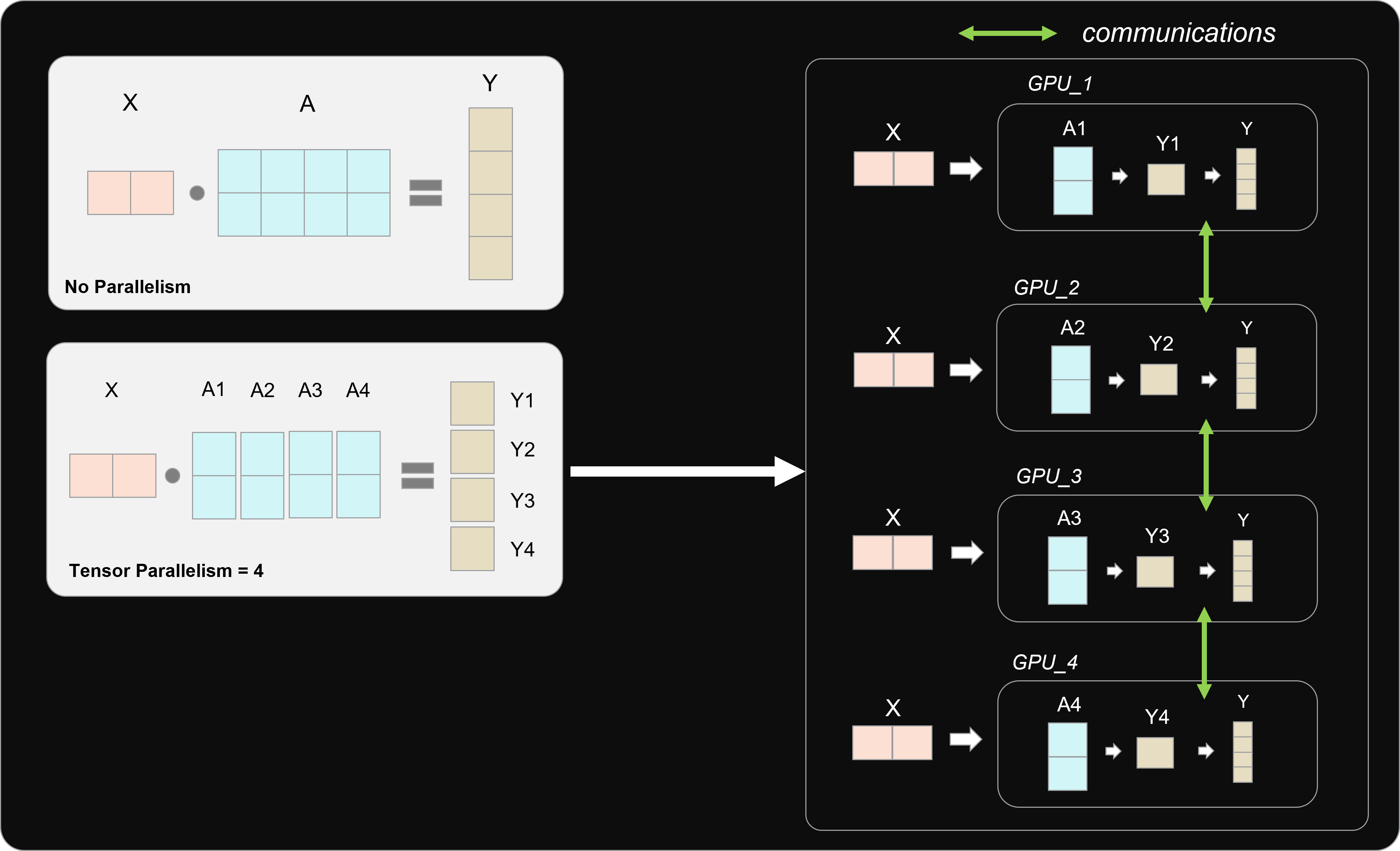
The primary communication primitive used in TP is all-reduce. This is a collective operation: all GPUs in the tensor-parallel group participate. They each contribute their partial result, the results are summed (or another operation is applied), and the final, identical sum is distributed back to all participating GPUs.
The Evolution of Multi-GPU Inference in vLLM | Ray Summit 2024
This clip from a vLLM presentation at Ray Summit 2024 gives a clear, practical walkthrough of how tensor parallelism works in an MLP layer and why it necessitates an all-reduce.
Watch the segment from 7:04 to 10:44. The speaker diagrams how sharding the MLP weights leads to partial results that can be multiplied locally but then require a final all-reduce to produce the correct layer output. Pay attention to the conclusion: TP improves latency but requires high communication overhead.
Let's summarize the communication characteristics of Tensor Parallelism:
- Operation:
all-reduce(collective). - Frequency: High. Occurs multiple times within each transformer layer (e.g., in both the attention and MLP blocks) for both the forward and backward passes.
- Message Size: Small to Medium. The messages are fractions of activation tensors, not the full model's parameters.
- Sensitivity: Highly sensitive to both latency () and bandwidth (). The high frequency of operations means the latency cost () adds up quickly.
- Bottleneck: The sheer number of synchronous, collective calls. This is why TP is almost exclusively used within a single node where it can leverage the ultra-low latency and high bandwidth of NVLink. Attempting TP across nodes with higher-latency InfiniBand or Ethernet is often prohibitively slow.
3. The Communication Pattern of Pipeline Parallelism
Pipeline Parallelism (PP), as you know from the previous lessons, partitions the model between layers. GPUs are arranged in a series of stages.
The communication here is much simpler. Stage i performs its computations and then needs to pass its resulting activations to stage i+1. This is a direct transfer between two specific GPUs.
The primary communication primitive is send/recv. This is a point-to-point operation.
The Evolution of Multi-GPU Inference in vLLM | Ray Summit 2024
Let's return to the vLLM presentation, which now contrasts PP with TP.
Watch from 11:32 to 13:20. The speaker explains how PP uses a send/recv paradigm. Note the key takeaway: PP has much lower communication overhead than TP but is prone to execution bubbles.
Let's summarize the communication characteristics of Pipeline Parallelism:
- Operation:
send/recv(point-to-point). - Frequency: Low. Occurs once per micro-batch at each stage boundary.
- Message Size: Medium to Large. The message is the full activation tensor for a micro-batch at a given layer.
- Sensitivity: Primarily sensitive to bandwidth (). Because messages are large and transfers are infrequent, the startup latency () is less of a factor compared to the time it takes to transfer the large activation tensor.
- Bottleneck: Not the communication time itself, but the pipeline bubble (compute idle time) created by waiting for the communication to complete.
4. Comparing the Overheads: A Tale of Two Bottlenecks
We now have a clear picture of two different approaches with two different bottlenecks.
| Strategy | Primary Operation | Communication Scope | Frequency | Message Size | Primary Bottleneck |
|---|---|---|---|---|---|
| Tensor Parallelism | all-reduce |
Collective (All TP GPUs) | High | Small/Medium | Communication overhead (latency & bandwidth) |
| Pipeline Parallelism | send/recv |
Point-to-Point (Adjacent GPUs) | Low | Medium/Large | Compute idle time (the pipeline bubble) |
This table, adapted from the apxml.com resource, is the central mental model for this lesson.
- TP trades increased communication for better compute utilization. It keeps all GPUs busy on the same layer but pays a high price in network traffic.
- PP trades compute utilization for less communication. It has a much lighter communication pattern but pays a price in idle GPU time (the bubble).

5. The Hybrid Solution: A Practical Rule of Thumb
Given these opposing characteristics, the industry has converged on a clear best practice: combine them.
The strategy, articulated in foundational papers like Megatron-LM and implemented in frameworks like vLLM, is:
- Use Tensor Parallelism to scale up to the number of GPUs within a single node, taking advantage of high-bandwidth, low-latency NVLink.
- Use Pipeline Parallelism to scale across nodes, using the more efficient point-to-point communication pattern over the slower inter-node network.
Training LLMs at Scale - Deepak Narayanan | Stanford MLSys #83
This segment from a Stanford MLSys seminar provides empirical evidence for this hybrid strategy. The speaker analyzes the performance of different TP and PP combinations and shows exactly where the sweet spot lies.
Watch from 15:25 to 22:40. The speaker introduces an analytical model showing that as TP size increases, the pipeline bubble decreases. But this comes at a cost: the all-reduce communication overhead of TP. The graph at 19:00 is crucial: it shows the measured throughput for a 162B parameter model on 64 GPUs. Throughput is low for small TP sizes (due to cross-node all-reduce) and for large PP sizes (due to large pipeline bubbles). The peak performance is at a TP size of 8 (the number of GPUs in one node) and a PP size of 8.
The video demonstrates the core trade-off perfectly. Increasing TP size reduces the pipeline bubble but increases communication overhead. The optimal point is right at the node boundary, where all-reduce stays on fast NVLink.
The seminal paper "Efficient Large-Scale Language Model Training on GPU Clusters..." (Megatron-LM) codifies this as "Takeaway #1":
When considering different forms of model parallelism, tensor model parallelism should generally be used up to degree 𝑔 when using 𝑔-GPU servers, and then pipeline model parallelism can be used to scale up to larger models across servers. (Section 3.2, resource ID LINK)
This principle is directly applicable to your work. If you need to serve a model that requires 16 GPUs, and you have two 8-GPU servers, the default configuration would be TP=8, PP=2.
The Evolution of Multi-GPU Inference in vLLM | Ray Summit 2024
Finally, let's hear this rule of thumb stated explicitly in the context of a production inference server.
Watch the Q&A segment from 27:12 to 28:30. The speaker gives direct guidance: use TP within a node and PP when you go multi-node or when you are on cheaper GPUs without NVLink. The questioner confirms the understanding with a 400B model example: on two nodes, you'd use TP=8 and PP=2. This is a perfect, concrete application of our analysis.
Conclusion
In this lesson, you've dissected the communication patterns that define tensor and pipeline parallelism, moving beyond the compute-centric view of the pipeline bubble. You now have a robust framework for reasoning about these critical trade-offs.
Key Takeaways:
- Tensor Parallelism (TP) relies on frequent, collective
all-reduceoperations. Its high communication overhead makes it best suited for fast intra-node interconnects like NVLink. - Pipeline Parallelism (PP) uses infrequent, point-to-point
send/recvoperations. Its lighter communication profile makes it suitable for scaling across slower inter-node links, but it introduces compute inefficiency via the pipeline bubble. - The fundamental trade-off is TP's communication overhead vs. PP's compute under-utilization.
- The industry-standard solution is a hybrid model: use TP up to the node boundary, and PP to connect nodes. This minimizes expensive cross-node
all-reducewhile keeping the pipeline depth (and thus the bubble) manageable.
Preview of the Next Lesson:
You've now analyzed the compute and communication trade-offs of TP and PP in isolation and in combination. In the next lesson, we will put it all together. You will be tasked to determine an optimal parallelism configuration (e.g., hybrid TP/PP) for serving a 70B model on a 4xH100 cluster based on memory and communication trade-offs. This will require you to apply the principles from this and previous lessons to a concrete system design problem, balancing model memory, KV cache, compute utilization, and network overhead.